📝 Week 8 - Lab Intro#
In this lab introduction we will briefly review how Arrays and broadcasting for this lab
import numpy as np
import matplotlib.pyplot as plt
Creating Arrays#
Creating an array of zeros,#
We often want an empty array to begin iterative calculations. We can use np.zeros() to create an array of zeros. If you forget what the inputs are, hover over the function, and press shift + tab to view the docstring.
print(np.zeros(10))
[0. 0. 0. 0. 0. 0. 0. 0. 0. 0.]
print(np.zeros((2,3)))
[[0. 0. 0.]
 [0. 0. 0.]]
Creating an array with equal spacing#
To make an array with equal spacing, use np.linspace(). This method can only create 1D arrays.
print(np.linspace(0,1))
[0.         0.02040816 0.04081633 0.06122449 0.08163265 0.10204082
 0.12244898 0.14285714 0.16326531 0.18367347 0.20408163 0.2244898
 0.24489796 0.26530612 0.28571429 0.30612245 0.32653061 0.34693878
 0.36734694 0.3877551  0.40816327 0.42857143 0.44897959 0.46938776
 0.48979592 0.51020408 0.53061224 0.55102041 0.57142857 0.59183673
 0.6122449  0.63265306 0.65306122 0.67346939 0.69387755 0.71428571
 0.73469388 0.75510204 0.7755102  0.79591837 0.81632653 0.83673469
 0.85714286 0.87755102 0.89795918 0.91836735 0.93877551 0.95918367
 0.97959184 1.        ]
The default number of points is 50. If we want to change the number of points, we can use input num=...
print(np.linspace(0,1,num=10))
[0.         0.11111111 0.22222222 0.33333333 0.44444444 0.55555556
 0.66666667 0.77777778 0.88888889 1.        ]
If we want to exclude the endpoint, we can use input endpoint=False.
print(np.linspace(0,1,num=10,endpoint=False))
[0. 0.1 0.2 0.3 0.4 0.5 0.6 0.7 0.8 0.9]
Create array from list#
num_list = [0,3,4,5,7]
arr = np.array(num_list)

print(arr, type(num_list), type(arr))
[0 3 4 5 7] <class 'list'> <class 'numpy.ndarray'>
Broadcasting#
Numpy arrays can infer how to distribute a calculation across axes. This is called broadcasting. For example, let’s try some basic operations
test_array = np.zeros(5)
print(test_array)
[0. 0. 0. 0. 0.]
test_array = test_array+1
print(test_array)
[1. 1. 1. 1. 1.]
test_array = test_array * 6
print(test_array)
[6. 6. 6. 6. 6.]
Arrays are important because we can’t perform these operations on lists. You will get a “TypeError”
test_list = [0,0,0,0,0]
test_list = test_list+1
---------------------------------------------------------------------------
TypeError                                 Traceback (most recent call last)
Cell In[21], line 2
      1 test_list = [0,0,0,0,0]
----> 2 test_list = test_list+1

TypeError: can only concatenate list (not "int") to list
What happens when we perform operations on arrays of different shapes?#
test_array = np.ones(5)
print(test_array)
[1. 1. 1. 1. 1.]
test_linspace_array = np.linspace(0,1,num=10,endpoint=False)
print(test_linspace_array)
[0. 0.1 0.2 0.3 0.4 0.5 0.6 0.7 0.8 0.9]
test_array + test_linspace_array
---------------------------------------------------------------------------
ValueError                                Traceback (most recent call last)
Cell In[24], line 1
----> 1 test_array + test_linspace_array

ValueError: operands could not be broadcast together with shapes (5,) (10,)
We see that need to perform operations on arrays with similiar shapes
np functions and broadcasting#
Many numpy function will automatically broadcast depending on the shape of your input
np.sin(np.pi/2)
1.0
test_linspace_array = np.linspace(0,1,num=10,endpoint=False)
print(test_linspace_array.shape)

print(np.sin(np.pi * test_linspace_array))
(10,)
[0.         0.30901699 0.58778525 0.80901699 0.95105652 1.
 0.95105652 0.80901699 0.58778525 0.30901699]
Plotting arrays#
To plot, we can use the plt.plot(x_array,y_array)
We can also add a title and axis labels using plt.title(), plt.xlabel() and plt.ylable()
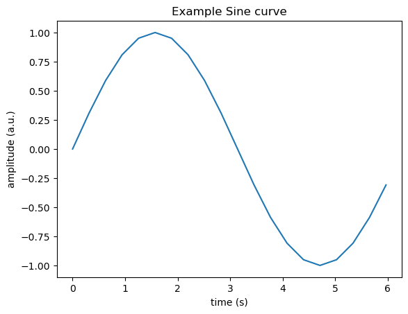
t = np.linspace(0,2*np.pi,num=20,endpoint=False)
y = np.sin(t)

plt.plot(t,y) # line plot
#plt.scatter(t,y) #scatter plot
plt.title('Example Sine curve')
plt.xlabel('time (s)')
plt.ylabel('amplitude (a.u.)')
Text(0, 0.5, 'amplitude (a.u.)')