# Initialize Otter
import otter
grader = otter.Notebook("lab9-pollutant.ipynb")
Lab 9: Pollutant Triangulation#
This lab uses classes to solve a problem involving pollutant triangulation.
Entering Your Information for Credit#
To receive credit for assignments it is important we can identify your work from others. To do this we will ask you to enter your information in the following code block.
Before you begin#
Run the block of code at the top of the notebook that imports and sets up the autograder. This will allow you to check your work.
# Please provide your first name, last name, Drexel ID, and Drexel email. Make sure these are provided as strings. "STRINGS ARE TEXT ENCLOSED IN QUOTATION MARKS."

# In the assignments you will see sections of code that you need to fill in that are marked with ... (three dots). Replace the ... with your code.
first_name = ...
last_name = ...
drexel_id = ...
drexel_email = ...
grader.check("q0-Checking-Your-Name")
import drexel_jupyter_logger
import matplotlib.pyplot as plt
import numpy as np
# import IPython.display as ipd
Use triangulation to locate pollutant source#
Triangulation, such as used in GPS positioning uses three points and two distances to calculate the location of an unknown point.
Now, let’s suppose that the unknown point is actually a point source for some pollutant X, and at time 0 it releases a burst of Chemical X. Assume no wind, and that X diffuses freely from its release point.
Suppose that we have measurement devices at the three points 1, 2, and 3 that track the concentration of X as a function of time, and that the concentration of X is detected to peak at times \(t_1\), \(t_2\), and \(t_3\), at each point, respectively. Can we determine the location of the evil point source?
Task 1: Make a class for point in pollutant system#
In this system, we have collected data at points \((x_1,y_1)\), \((x_2,y_2)\), and \((x_3,y_3)\), at times \(t_1\), \(t_2\), and \(t_3\) respectively. We would like to encapsulate this data, and find a way to extract distance using the diffusivity of \(X\) \((D_X)\).
Let’s make the assumption that the time intervals \((t_i)\) scale with the square of the distance \((d_i)\) divided by the diffusivity of \(X\) \((D_X)\):
We can express the diffusivity using the following diffusion constant:
That satisfies the conditions
Write python code to do the following:
Define a class called
PointDefine the class constructor to accept as argument the floats
x,y,t, in that order. Make sure your parameters are in the right order! Store each value in a data member, so that they can be used in other methods.Define a method called
diffusion_distancewhich accepts as input the constantK, and returns the distance calculated using the Point memberself.t.
Your code replaces the prompt: ...
...

# Create point objects P1, P2, P3
Pt1 = Point(0,1,1)
Pt2 = Point(1,0,2)
Pt3 = Point(2,3,2)

print(f'Members of P1: ({Pt1.x},{Pt1.y},{Pt1.t})')

# Solve diffusion distance
dist1 = Pt1.diffusion_distance(2.5)
print('Calculate diffusion distance of P1:', dist1)

# Plot P1,P2,P3
plt.clf()
plt.plot(Pt1.x,Pt1.y,'ro')
plt.plot(Pt2.x,Pt2.y,'b*')
plt.plot(Pt3.x,Pt3.y,'k+')
plt.grid()
grader.check("task1-Point-class")
Task 2: Make a class to triangulate between 3 points#
In the previous task, we determined how to calculate the distance between a point and a pollutant source, given diffusion constant \(K\) and time \(t\). How can we use this information to find the location of a pollutant source?
Intro to Triangulation
Triangulation is the process of locating an unknown point given two know points, and two known distances.
Consider two points \((x_1,y_1)\) and \((x_2,y_2\)).
Let \((x,y)\) be an unknown point whose respective distances to the two points, \(d_1\) and \(d_2\), are known. The Pythagorean theorem allows us to express \(x\) and \(y\) (the coordinates of the unknown point) in terms of \((x_1,y_1)\), \((x_2,y_2)\), \(d_1\), and \(d_2\): $\( d_1^{2} = (x - x_1)^{2} + (y - y_1)^{2}\)\( \)\( d_2^{2} = (x - x_2)^{2} + (y - y_2)^{2}\)$
Inverting these two formulae to make them explicit in \(x\) and \(y\) is really a lot of fun, but it takes a while. Here is the final result: $\( x_{\pm} = \frac{1}{2(1 + b^2)} \left[ 2 [x_1 - b(a - y_1)] \pm [4(b(a - y_1) - x_1)^2 - 4(1 + b^2)(x_1^{2} - d_1^{2} + (y_1 - a)^{2})]^{\frac{1}{2}} \right] \)\( \)\( y_{\pm} = a + bx_{\pm} \)$
where $\( a = \frac{d_1^{2} - d_2^{2} - [(x_1^{2} + y_1^{2}) - (x_2^{2} + y_2^{2})]}{2(y_2 - y_1)} \)$
and $\( b = - \frac{x_2 - x_1}{y_2 - y_1} \)$
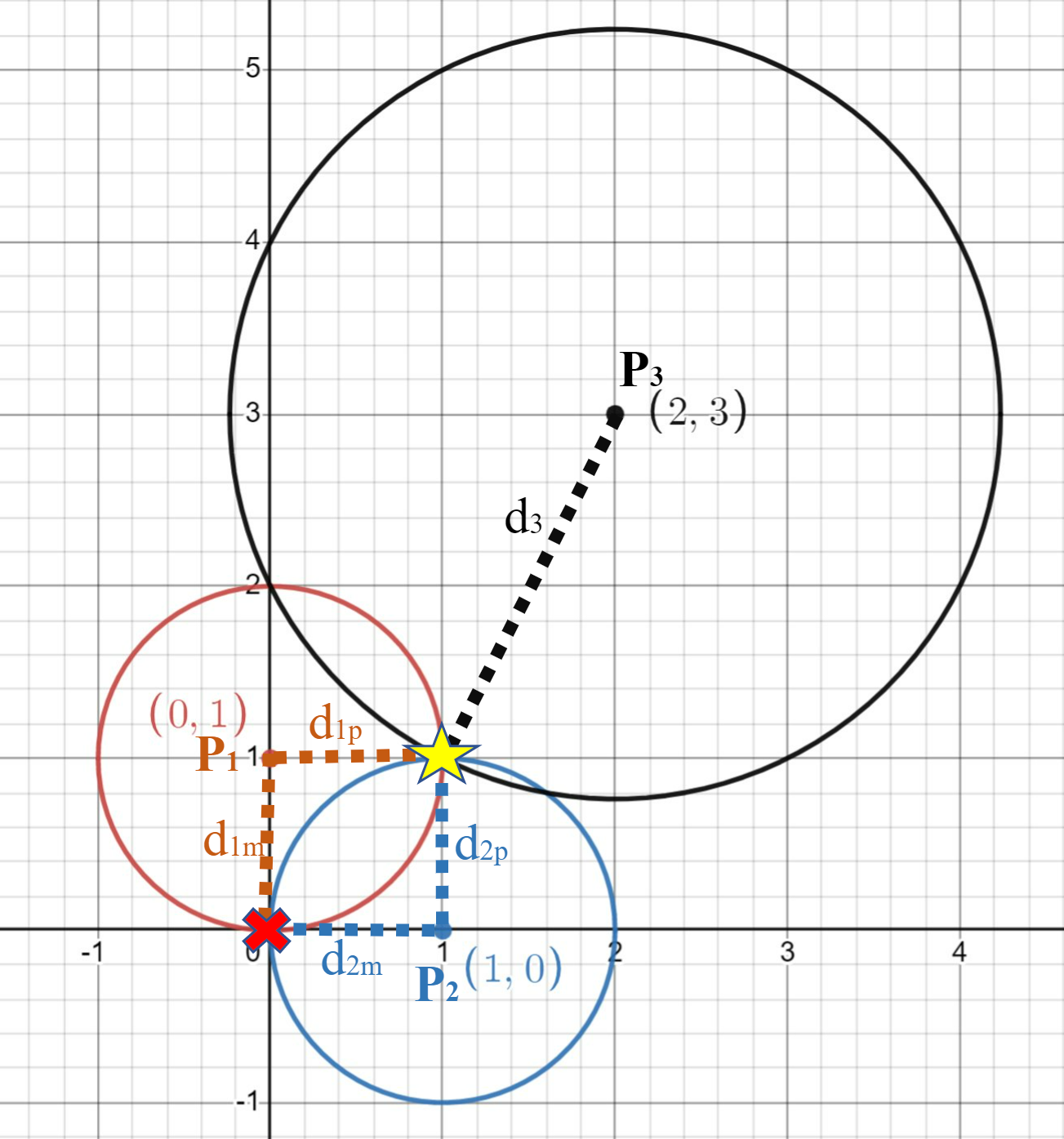
Note that the two possible values for \(x\), \(x_+\) and \(x_-\), arise from the positive and negative sense of the square root, and the value of \(y\) derives from its particular \(x\). So because of the power of 2 in the Pythagorean theorem, we find that there are two possible points, \((x_+, y_+)\) and \((x_-, y_-)\), that are each \(d_1\) from \((x_1, y_1)\) and \(d_2\) from \((x_2, y_2)\). These are shown by the star and cross in the figure below.
“Triangulation” refers to the fact that we need a third known point to decide which of \((x_+, y_+)\) and \((x_-, y_-)\) is our sought-after point. We would like the final unknown point to be the one that is closer to \((x_3, y_3)\), shown as the star in the figure below:
Write a python code to do the following:
Create a class
Point_SystemDefine the class constructor to accept as argument the Point objects
P1,P2, andP3, in that order. Store each value in a data member, so that they can be used in other methods.Define a method called
pythagoraswhich accepts as input andx1,y1,x2,y2, which are the coordinates of the pointsself.P1andself.P2. This method should return the euclidean distance between the two points.Define a method called
a_bwhich accepts as input the distances between a point andself.P1andself.P2, asd1andd2respectively. This method should return the tuplea,b, calculated with the equation above.Define a method called
x_ywhich accepts as input the distances between a point andself.P1andself.P2, asd1andd2respectively. This method should return the tuplexm,ym,xp,yp, which are the “minus” coordinates(xm,ym)and “plus” coordinates(xp,yp)of a point, calculated with the equation above.Define a method called
triangulatewhich accepts as input the distances between a point andself.P1andself.P2, asd1andd2respectively. This method should return the tuplexf,yf, the coordinate closest to the third point,self.P3.Calculate the potential coordinates of a point the distance
d1from pointself.P1, and distanced2fromself.P2using the method we defined,x_y. Assign this to the variablesxm,ym,xp,yp.Assign a variable
d3mto be the distance between the estimated “minus” coordinatexm,ymand the pointself.P3Assign a variable
d3pto be the distance between the estimated “plus” coordinatexp,ypand the pointself.P3Check whether
d3mord3pis smaller. Set the corresponding \((x,y)\) coordinates to variablesxf,yfReturn the final triangulated coordinates,
xf,yf.
Your code replaces the prompt: ...
...

# create Point object P1, P2, P3
Pt1 = Point(0,1,1)
Pt2 = Point(1,0,2)
Pt3 = Point(2,3,2)

# Create Point_System object System, using P1, P2, P3 as inputs
System = Point_System(Pt1,Pt2,Pt3)

# Plot points Point_System objects P1, P2, P3
plt.clf()
plt.plot(System.P1.x,System.P1.y,'ro')
plt.plot(System.P2.x,System.P2.y,'b*')
plt.plot(System.P3.x,System.P3.y,'k+')
plt.grid()
grader.check("task2-System-class")
Task 3: Predict location of pollutant and diffusivity#
Our system consists of three points, \(P_1=(-4,7), P_2=(-5,-6), P_3=(9,1)\), and a pollution source with unknown coordinates and diffusion coefficient \(K\). After the release of the chemical, the pollution peaked at the three points at times \(300,400,500\) respectively. We want to estimate \(K\) and the coordinates of the pollutant.
We can achieve this using an iterative process that slowly modifies K by multiplying it by a change factor \(\epsilon\), and recalculates the predicted coordinates. The process will repeat until K is modified by less than a factor of \(10^{-6}\) (In other words, the code runs if \(|K-K\epsilon|>K10^{-6}\)). Write a code to do the following:
Create
PointobjectsP1,P2andP3, initialized with the coordinates and times given aboveCreate a
Point_SystemobjectSysinitialized with point objectsP1,P2andP3.We are satisfied with our guess when K changes by less than a factor of \(10^{-6}\) per iteration. Assign this value to variable
criteria. This variable will not change!Assign 1.0 as our initial guess of
KAssign
criteria\(10^{-6}\) as our initial change factor,epsilonWrite a loop that runs until K is modified by less than a factor of \(10^{-6}\). Inside, the loop performs the following steps:
Compute the distances of
d1,d2, andd3with the given values of K.Use triangulation to find the points
xf,yf, which are the correct distance from P1 and P2, and closest to P3.Compute the distance
d3_, which is the distance between(xf,yf)andP3.Calculate our change factor
epsilonusing the following equation: \(\epsilon=\sqrt{d_{3\ guess}/d_{3\ true}}\).print the values of
d3_,d3,epsilon, andK.Change \(K\) to \(K\epsilon\).
Your code replaces the prompt: ...
# Define Variables
...

# create loop that modifies K
...

# Print the estimated diffusivity
print(f'Diffusivity of X is about {K**2:.3f}')
# Print the estimated location of the point source
print(f'Evil point source is ({xf:.3f},{yf:.3f})')
grader.check("task3-predict")
Take a look at the points and the pollutant source
import matplotlib.pyplot as plt

plt.clf()
plt.xlim([min([P1.x,P2.x,P3.x,xf])-1,max([P1.x,P2.x,P3.x,xf])+1])
plt.ylim([min([P1.y,P2.y,P3.y,yf])-1,max([P1.y,P2.y,P3.y,yf])+1])
plt.plot(P1.x,P1.y,'bo')
plt.plot(P2.x,P2.y,'go')
plt.plot(P3.x,P3.y,'co')
plt.plot(xf,yf,'ro')

plt.plot([P1.x,xf],[P1.y,yf],'k-')
plt.plot([P2.x,xf],[P2.y,yf],'k-')
plt.plot([P3.x,xf],[P3.y,yf],'k-')

plt.annotate('P1',xy=(P1.x,P1.y))
plt.annotate('P2',xy=(P2.x,P2.y))
plt.annotate('P3',xy=(P3.x,P3.y))
plt.annotate('evil point source',xy=(xf,yf))
plt.show()
Submitting Your Assignment#
To submit your assignment please use the following link the assignment on GitHub classroom.
Use this link to navigate to the assignment on GitHub classroom.
If you need further instructions on submitting your assignment please look at Lab 1.
Viewing your score#
It is your responsibility to ensure that your grade report shows correctly. We can only provide corrections to grades if a grading error is determined. If you do not receive a grade report your grade has not been recorded. It is your responsibility either resubmit the assignment correctly or contact the instructors before the assignment due date.
Each .ipynb file you have uploaded will have a file with the name of your file + Grade_Report.md. You can view this file by clicking on the file name. This will show you the results of the autograder.
We have both public and hidden tests. You will be able to see the score of both tests, but not the specific details of why the test passed or failed.
Note
In python and particularly jupyter notebooks it is common that during testing you run cells in a different order, or run cells and modify them. This can cause there to be local variables needed for your solution that would not be recreated on running your code again from scratch. Your assignment will be graded based on running your code from scratch. This means before you submit your assignment you should restart the kernel and run all cells. You can do this by clicking Kernel and selecting Restart and Run All. If you code does not run as expected after restarting the kernel and running all cells it means you have an error in your code.