Automatic Differentiation with torch.autograd
Contents
%matplotlib inline

import torch
Automatic Differentiation with torch.autograd#
When training neural networks, the most frequently used algorithm is back propagation. In this algorithm, parameters (model weights) are adjusted according to the gradient of the loss function with respect to the given parameter.
To compute those gradients, PyTorch has a built-in differentiation engine
called torch.autograd. It supports automatic computation of gradient for any
computational graph.
Consider the simplest one-layer neural network, with input x,
parameters w and b, and some loss function. It can be defined in
PyTorch in the following manner:
x = torch.ones(5)  # input tensor
y = torch.zeros(3)  # expected output
w = torch.randn(5, 3, requires_grad=True)
b = torch.randn(3, requires_grad=True)
z = torch.matmul(x, w) + b
loss = torch.nn.functional.binary_cross_entropy_with_logits(z, y)
Tensors, Functions and Computational graph#
This code defines the following computational graph:
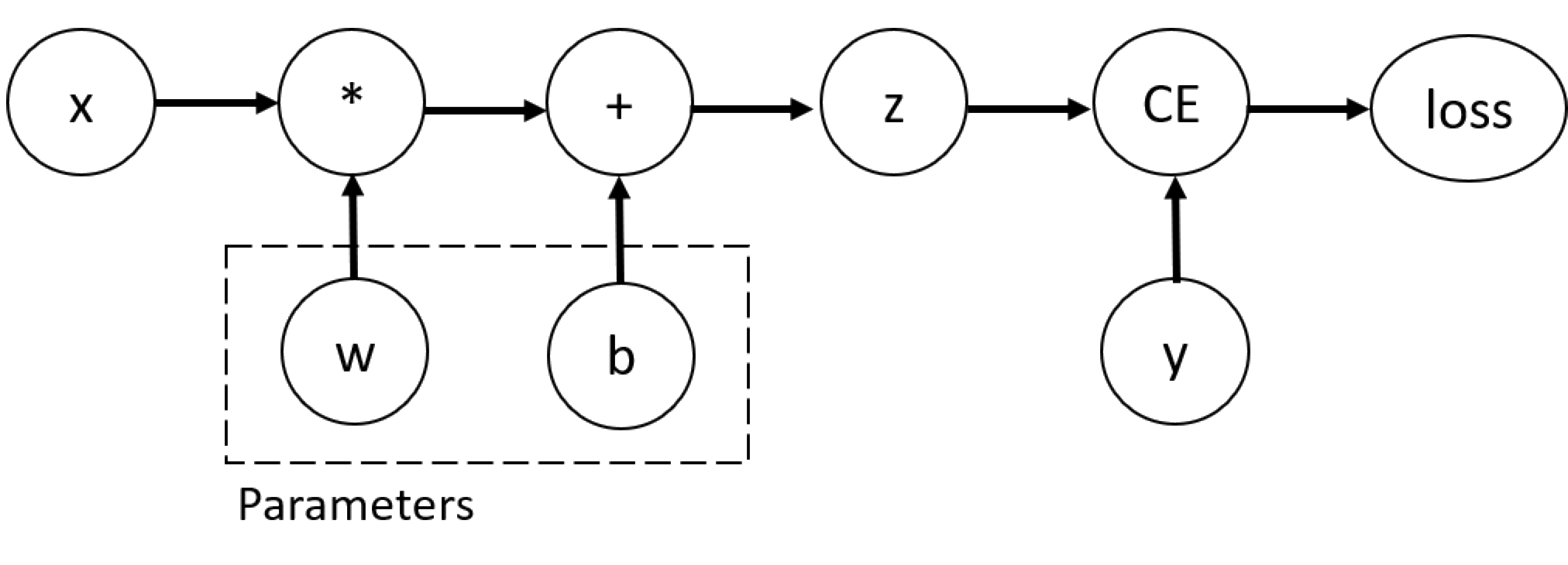
In this network, w and b are parameters, which we need to
optimize. Thus, we need to be able to compute the gradients of loss
function with respect to those variables. In order to do that, we set
the requires_grad property of those tensors.
Note
You can set the value of ``requires_grad`` when creating a tensor, or later by using ``x.requires_grad_(True)`` method.
A function that we apply to tensors to construct computational graph is
in fact an object of class Function. This object knows how to
compute the function in the forward direction, and also how to compute
its derivative during the backward propagation step. A reference to
the backward propagation function is stored in grad_fn property of a
tensor. You can find more information of Function in the
documentation.
print(f"Gradient function for z = {z.grad_fn}")
print(f"Gradient function for loss = {loss.grad_fn}")
Gradient function for z = <AddBackward0 object at 0x0000019F867730D0>
Gradient function for loss = <BinaryCrossEntropyWithLogitsBackward0 object at 0x0000019FE02BDC60>
Computing Gradients#
To optimize weights of parameters in the neural network, we need to
compute the derivatives of our loss function with respect to parameters,
namely, we need \(\frac{\partial loss}{\partial w}\) and
\(\frac{\partial loss}{\partial b}\) under some fixed values of
x and y. To compute those derivatives, we call
loss.backward(), and then retrieve the values from w.grad and
b.grad:
loss.backward()
print(w.grad)
print(b.grad)
tensor([[0.0511, 0.0101, 0.2891],
        [0.0511, 0.0101, 0.2891],
        [0.0511, 0.0101, 0.2891],
        [0.0511, 0.0101, 0.2891],
        [0.0511, 0.0101, 0.2891]])
tensor([0.0511, 0.0101, 0.2891])
Note
- We can only obtain the ``grad`` properties for the leaf nodes of the computational graph, which have ``requires_grad`` property set to ``True``. For all other nodes in our graph, gradients will not be available. - We can only perform gradient calculations using ``backward`` once on a given graph, for performance reasons. If we need to do several ``backward`` calls on the same graph, we need to pass ``retain_graph=True`` to the ``backward`` call.
Disabling Gradient Tracking#
By default, all tensors with requires_grad=True are tracking their
computational history and support gradient computation. However, there
are some cases when we do not need to do that, for example, when we have
trained the model and just want to apply it to some input data, i.e. we
only want to do forward computations through the network. We can stop
tracking computations by surrounding our computation code with
torch.no_grad() block:
z = torch.matmul(x, w) + b
print(z.requires_grad)

with torch.no_grad():
    z = torch.matmul(x, w) + b
print(z.requires_grad)
True
False
Another way to achieve the same result is to use the detach() method
on the tensor:
z = torch.matmul(x, w) + b
z_det = z.detach()
print(z_det.requires_grad)
False
There are reasons you might want to disable gradient tracking:
To mark some parameters in your neural network as frozen parameters. This is a very common scenario for finetuning a pretrained network
To speed up computations when you are only doing forward pass, because computations on tensors that do not track gradients would be more efficient.
More on Computational Graphs#
Conceptually, autograd keeps a record of data (tensors) and all executed operations (along with the resulting new tensors) in a directed acyclic graph (DAG) consisting of Function_ objects. In this DAG, leaves are the input tensors, roots are the output tensors. By tracing this graph from roots to leaves, you can automatically compute the gradients using the chain rule.
In a forward pass, autograd does two things simultaneously:
run the requested operation to compute a resulting tensor
maintain the operation’s gradient function in the DAG.
The backward pass kicks off when .backward() is called on the DAG
root. autograd then:
computes the gradients from each
.grad_fn,accumulates them in the respective tensor’s
.gradattributeusing the chain rule, propagates all the way to the leaf tensors.
Note
**DAGs are dynamic in PyTorch** An important thing to note is that the graph is recreated from scratch; after each ``.backward()`` call, autograd starts populating a new graph. This is exactly what allows you to use control flow statements in your model; you can change the shape, size and operations at every iteration if needed.