import seaborn as sns
import pandas as pd


from sklearn import set_config
from sklearn.model_selection import cross_val_score, train_test_split
from sklearn.compose import ColumnTransformer
from sklearn.compose import make_column_selector as selector
from sklearn.preprocessing import OrdinalEncoder
from sklearn.pipeline import Pipeline
from sklearn.model_selection import GridSearchCV
from sklearn.ensemble import HistGradientBoostingClassifier

set_config(display="diagram")

Hyperparameter tuning by grid-search

There are many parameters that need to be tuned when building a machine-learning model.

• It is non-intuitive what these parameters should be

Example: Adults Census Data

This is a dataset that contains information from the 1994 Census. The goal is to predict if a person makes more than $50,000 per year based on their demographic information.

Step 1: Load the Data

adult_census = pd.read_csv("./data/adult-census.csv")

Step 2: Visualize and Clean the Data

We extract the column containing the target.

target_name = "class"
target = adult_census[target_name]
target

0         <=50K
1         <=50K
2          >50K
3          >50K
4         <=50K
          ...  
48837     <=50K
48838      >50K
48839     <=50K
48840     <=50K
48841      >50K
Name: class, Length: 48842, dtype: object

We drop from our data the target and the "education-num" column which duplicates the information from the "education" column.

data = adult_census.drop(columns=[target_name, "education-num"])
data.head()

	age	workclass	education	marital-status	occupation	relationship	race	sex	capital-gain	capital-loss	hours-per-week	native-country
0	25	Private	11th	Never-married	Machine-op-inspct	Own-child	Black	Male	0	0	40	United-States
1	38	Private	HS-grad	Married-civ-spouse	Farming-fishing	Husband	White	Male	0	0	50	United-States
2	28	Local-gov	Assoc-acdm	Married-civ-spouse	Protective-serv	Husband	White	Male	0	0	40	United-States
3	44	Private	Some-college	Married-civ-spouse	Machine-op-inspct	Husband	Black	Male	7688	0	40	United-States
4	18	?	Some-college	Never-married	?	Own-child	White	Female	0	0	30	United-States

Step 3: Test Train Split

Once the dataset is loaded, we split it into training and testing sets.

data_train, data_test, target_train, target_test = train_test_split(
    data, target, random_state=42)

Step 4: Building a Pipeline

Within Scikit-learn there are tools to build a pipeline to automate preprocessing and data analysis.

We will define a pipeline. It will handle both numerical and categorical features.

The first step is to select all the categorical columns.

categorical_columns_selector = selector(dtype_include=object)
categorical_columns = categorical_columns_selector(data)

Here we will use a tree-based model as a classifier (i.e. HistGradientBoostingClassifier). That means:

• Numerical variables don’t need scaling;

• Categorical variables can be dealt with by an OrdinalEncoder even if the coding order is not meaningful;

• For tree-based models, the OrdinalEncoder avoids having high-dimensional representations.

We now build our OrdinalEncoder by passing it to the known categories.

categorical_preprocessor = OrdinalEncoder(handle_unknown="use_encoded_value",
                                          unknown_value=-1)

We then use a ColumnTransformer to select the categorical columns and apply the OrdinalEncoder to them.

• The ColumnTransformer applies a transformation to the columns of a Pandas dataframe.

preprocessor = ColumnTransformer([
    ('cat_preprocessor', categorical_preprocessor, categorical_columns)],
    remainder='passthrough', sparse_threshold=0)

Finally, we use a tree-based classifier (i.e. histogram gradient-boosting) to predict whether or not a person earns more than 50 k$ a year.

model = Pipeline([
    ("preprocessor", preprocessor),
    ("classifier",
     HistGradientBoostingClassifier(random_state=42, max_leaf_nodes=4))])
model

Pipeline(steps=[('preprocessor',
                 ColumnTransformer(remainder='passthrough', sparse_threshold=0,
                                   transformers=[('cat_preprocessor',
                                                  OrdinalEncoder(handle_unknown='use_encoded_value',
                                                                 unknown_value=-1),
                                                  ['workclass', 'education',
                                                   'marital-status',
                                                   'occupation', 'relationship',
                                                   'race', 'sex',
                                                   'native-country'])])),
                ('classifier',
                 HistGradientBoostingClassifier(max_leaf_nodes=4,
                                                random_state=42))])

In a Jupyter environment, please rerun this cell to show the HTML representation or trust the notebook.
On GitHub, the HTML representation is unable to render, please try loading this page with nbviewer.org.

Step 5: Tuning the Model Using GridSearch

• GridSearchCV is a scikit-learn class that implements a very similar logic with less repetitive code.

Let’s see how to use the GridSearchCV estimator for doing such a search. Since the grid search will be costly, we will only explore the combination learning rate and the maximum number of nodes.

%%time
param_grid = {
    'classifier__learning_rate': (0.01, 0.1, 1, 10),
    'classifier__max_leaf_nodes': (3, 10, 30)}
model_grid_search = GridSearchCV(model, param_grid=param_grid,
                                 n_jobs=2, cv=2)
model_grid_search.fit(data_train, target_train)

CPU times: total: 11.5 s
Wall time: 5.95 s

GridSearchCV(cv=2,
             estimator=Pipeline(steps=[('preprocessor',
                                        ColumnTransformer(remainder='passthrough',
                                                          sparse_threshold=0,
                                                          transformers=[('cat_preprocessor',
                                                                         OrdinalEncoder(handle_unknown='use_encoded_value',
                                                                                        unknown_value=-1),
                                                                         ['workclass',
                                                                          'education',
                                                                          'marital-status',
                                                                          'occupation',
                                                                          'relationship',
                                                                          'race',
                                                                          'sex',
                                                                          'native-country'])])),
                                       ('classifier',
                                        HistGradientBoostingClassifier(max_leaf_nodes=4,
                                                                       random_state=42))]),
             n_jobs=2,
             param_grid={'classifier__learning_rate': (0.01, 0.1, 1, 10),
                         'classifier__max_leaf_nodes': (3, 10, 30)})

In a Jupyter environment, please rerun this cell to show the HTML representation or trust the notebook.
On GitHub, the HTML representation is unable to render, please try loading this page with nbviewer.org.

Step 6: Validation of the Model

Finally, we will check the accuracy of our model using the test set.

accuracy = model_grid_search.score(data_test, target_test)
print(
    f"The test accuracy score of the grid-searched pipeline is: "
    f"{accuracy:.2f}"
)

The test accuracy score of the grid-searched pipeline is: 0.88

Warning

Be aware that the evaluation should normally be performed through cross-validation by providing model_grid_search as a model to the cross_validate function.

Here, we used a single train-test split to evaluate model_grid_search. If interested you can look into more detail about nested cross-validation, when you use cross-validation both for hyperparameter tuning and model evaluation.

The GridSearchCV estimator takes a param_grid parameter which defines all hyperparameters and their associated values. The grid search will be in charge of creating all possible combinations and testing them.

The number of combinations will be equal to the product of the number of values to explore for each parameter (e.g. in our example 4 x 3 combinations). Thus, adding new parameters with their associated values to be explored become rapidly computationally expensive.

Once the grid search is fitted, it can be used as any other predictor by calling predict and predict_proba. Internally, it will use the model with the best parameters found during the fit.

Get predictions for the 5 first samples using the estimator with the best parameters.

model_grid_search.predict(data_test.iloc[0:5])

array([' <=50K', ' <=50K', ' >50K', ' <=50K', ' >50K'], dtype=object)

You can know about these parameters by looking at the best_params_ attribute.

print(f"The best set of parameters is: "
      f"{model_grid_search.best_params_}")

The best set of parameters is: {'classifier__learning_rate': 0.1, 'classifier__max_leaf_nodes': 30}

In addition, we can inspect all results which are stored in the attribute cv_results_ of the grid-search. We will filter some specific columns from these results.

cv_results = pd.DataFrame(model_grid_search.cv_results_).sort_values(
    "mean_test_score", ascending=False)
cv_results.head()

	mean_fit_time	std_fit_time	mean_score_time	std_score_time	param_classifier__learning_rate	param_classifier__max_leaf_nodes	params	split0_test_score	split1_test_score	mean_test_score	std_test_score	rank_test_score
5	0.5155	0.057500	0.086500	0.001500	0.1	30	{'classifier__learning_rate': 0.1, 'classifier...	0.868912	0.867213	0.868063	0.000850	1
4	0.3055	0.007500	0.085500	0.004500	0.1	10	{'classifier__learning_rate': 0.1, 'classifier...	0.866783	0.866066	0.866425	0.000359	2
7	0.1005	0.001501	0.067499	0.003500	1	10	{'classifier__learning_rate': 1, 'classifier__...	0.858648	0.862408	0.860528	0.001880	3
6	0.1070	0.008000	0.068499	0.000499	1	3	{'classifier__learning_rate': 1, 'classifier__...	0.859358	0.859514	0.859436	0.000078	4
8	0.1240	0.012000	0.063500	0.002500	1	30	{'classifier__learning_rate': 1, 'classifier__...	0.855536	0.856129	0.855832	0.000296	5

Let us focus on the most interesting columns and shorten the parameter names to remove the "param_classifier__" prefix for readability:

# get the parameter names
column_results = [f"param_{name}" for name in param_grid.keys()]
column_results += [
    "mean_test_score", "std_test_score", "rank_test_score"]
cv_results = cv_results[column_results]

def shorten_param(param_name):
    if "__" in param_name:
        return param_name.rsplit("__", 1)[1]
    return param_name


cv_results = cv_results.rename(shorten_param, axis=1)
cv_results

	learning_rate	max_leaf_nodes	mean_test_score	std_test_score	rank_test_score
5	0.1	30	0.868063	0.000850	1
4	0.1	10	0.866425	0.000359	2
7	1	10	0.860528	0.001880	3
6	1	3	0.859436	0.000078	4
8	1	30	0.855832	0.000296	5
3	0.1	3	0.853266	0.000515	6
2	0.01	30	0.843330	0.002917	7
1	0.01	10	0.817832	0.001124	8
0	0.01	3	0.797166	0.000715	9
11	10	30	0.288200	0.050539	10
9	10	3	0.283476	0.003775	11
10	10	10	0.262564	0.006326	12

Step 7: Visualizing Hyperparameter Tuning

With only 2 parameters, we might want to visualize the grid search as a heatmap. We need to transform our cv_results into a dataframe where:

• the rows will correspond to the learning-rate values;

• the columns will correspond to the maximum number of leaf;

• the content of the dataframe will be the mean test scores.

pivoted_cv_results = cv_results.pivot_table(
    values="mean_test_score", index=["learning_rate"],
    columns=["max_leaf_nodes"])

pivoted_cv_results

max_leaf_nodes	3	10	30
learning_rate
0.01	0.797166	0.817832	0.843330
0.10	0.853266	0.866425	0.868063
1.00	0.859436	0.860528	0.855832
10.00	0.283476	0.262564	0.288200

We can use a heatmap representation to show the above dataframe visually.

ax = sns.heatmap(pivoted_cv_results, annot=True, cmap="YlGnBu", vmin=0.7,
                 vmax=0.9)
ax.invert_yaxis()

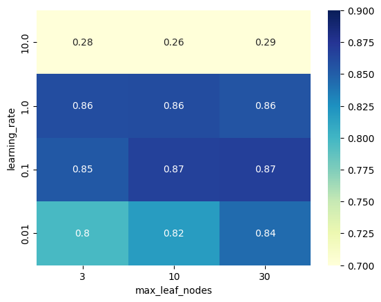
The above tables highlight the following things:

• for too high values of learning_rate, the generalization performance of the model is degraded and adjusting the value of max_leaf_nodes cannot fix that problem;

• outside of this pathological region, we observe that the optimal choice of max_leaf_nodes depends on the value of learning_rate;

• in particular, we observe a “diagonal” of good models with an accuracy close to the maximal of 0.87: when the value of max_leaf_nodes is increased, one should decrease the value of learning_rate accordingly to preserve a good accuracy.

For now, we will note that, in general, there are no unique optimal parameter setting: 4 models out of the 12 parameter configurations that reach the maximal accuracy (up to small random fluctuations caused by the sampling of the training set).