Introduction to SciPy
Contents
Introduction to SciPy#
SciPy is a collection of mathematical algorithms and convenience functions built on the NumPy extension of Python.
It adds significant power to the interactive Python session by providing the user high-level commands and classes for manipulating and visualizing data.
With SciPy, an interactive Python session becomes a data-processing and system-prototyping environment, rivaling systems such as MATLAB, IDL, Octave, R-Lab, and SciLab.
SciPy is organized into subpackages covering different scientific computing domains. These are summarized in the following table:
==================  ======================================================
Subpackage          Description
==================  ======================================================
`cluster`           Clustering algorithms
`constants`         Physical and mathematical constants
`fftpack`           Fast Fourier Transform routines
`integrate`         Integration and ordinary differential equation solvers
`interpolate`       Interpolation and smoothing splines
`io`                Input and Output
`linalg`            Linear algebra
`ndimage`           N-dimensional image processing
`odr`               Orthogonal distance regression
`optimize`          Optimization and root-finding routines
`signal`            Signal processing
`sparse`            Sparse matrices and associated routines
`spatial`           Spatial data structures and algorithms
`special`           Special functions
`stats`             Statistical distributions and functions
==================  ======================================================
Scipy.special#
The main feature of the scipy.special package is the definition of numerous special functions of mathematical physics. Available functions include airy, elliptic, bessel, gamma, beta, hypergeometric, parabolic cylinder, mathieu, spheroidal wave, struve, and kelvin.
Bessel functions of real order(jv, jn_zeros)#
Bessel functions are a family of solutions to Bessel’s differential equation with real or complex order alpha:
Among other uses, these functions arise in wave propagation problems, such as the vibrational modes of a thin drum head. Here is an example of a circular drum head anchored at the edge:
from scipy import special
import numpy as np


def drumhead_height(n, k, distance, angle, t):
    kth_zero = special.jn_zeros(n, k)[-1]
    return np.cos(t) * np.cos(n * angle) * special.jn(n, distance * kth_zero)


theta = np.r_[0 : 2 * np.pi : 50j]
radius = np.r_[0:1:50j]

x = np.array([r * np.cos(theta) for r in radius])
y = np.array([r * np.sin(theta) for r in radius])
z = np.array([drumhead_height(1, 1, r, theta, 0.5) for r in radius])
import matplotlib.pyplot as plt

fig = plt.figure()
ax = fig.add_axes(rect=(0, 0.05, 0.95, 0.95), projection="3d")
ax.plot_surface(x, y, z, rstride=1, cstride=1, cmap="RdBu_r", vmin=-0.5, vmax=0.5)
ax.set_xlabel("X")
ax.set_ylabel("Y")
ax.set_xticks(np.arange(-1, 1.1, 0.5))
ax.set_yticks(np.arange(-1, 1.1, 0.5))
ax.set_zlabel("Z")
plt.show()

Integration#
The scipy.integrate sub-package provides several integration techniques including an ordinary differential equation integrator. An overview of the module is provided by the help command:
General Integration#
The function quad is provided to integrate a function of one variable between two points. The points can be \(\pm\infty\) (\(\pm inf\)) to indicate infinite limits. For example, suppose you wish to integrate a bessel function jv(2.5, x) along the interval [0, 4.5].
import scipy.integrate as integrate
import scipy.special as special

result = integrate.quad(lambda x: special.jv(2.5, x), 0, 4.5)
result
(1.1178179380783253, 7.866317250224184e-09)
The first argument to quad is a “callable” Python object (i.e., a function, method, or class instance).
Notice the use of a lambda- function in this case as the argument.
The next two arguments are the limits of integration.
The return value is a tuple, with the first element holding the estimated integral value and the second element holding an upper bound on the error.
Optimization#
SciPy has a bunch of built-in fitting methods, which forms the framework for curve fitting and other more advanced optimization
You could take an entire course that discusses the details of these optimization methods
Generally, in machine learning, we have so many dimensions that it is possible to use simple optimizers
Example: Curve Fitting#
import matplotlib.pyplot as plt
from scipy.optimize import curve_fit
def func(x, a, b, c):
    return a * np.exp(-b * x) + c
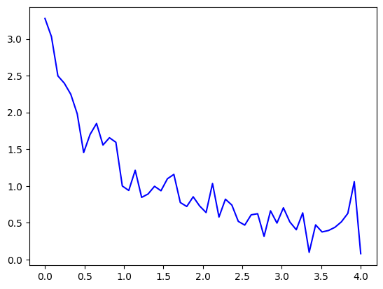
Define the noisy data to fit:
xdata = np.linspace(0, 4, 50)
y = func(xdata, 2.5, 1.3, 0.5)
rng = np.random.default_rng()
y_noise = 0.2 * rng.normal(size=xdata.size)
ydata = y + y_noise
plt.plot(xdata, ydata, "b-", label="data")
[<matplotlib.lines.Line2D at 0x207bba8a650>]
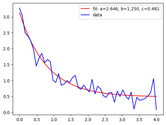
Fit for the parameters a, b, c of the function func:
popt, pcov = curve_fit(func, xdata, ydata)
popt
plt.plot(
    xdata,
    func(xdata, *popt),
    "r-",
    label="fit: a=%5.3f, b=%5.3f, c=%5.3f" % tuple(popt),
)
plt.plot(xdata, ydata, "b-", label="data")
plt.legend()
<matplotlib.legend.Legend at 0x207bcc26aa0>
Constrain the optimization to the region of 0 <= a <= 3, 0 <= b <= 1 and 0 <= c <= 0.5:
popt, pcov = curve_fit(func, xdata, ydata, bounds=(0, [3.0, 1.0, 0.5]))
popt
array([2.56993512, 1. , 0.37915003])
plt.plot(
    xdata,
    func(xdata, *popt),
    "g--",
    label="fit: a=%5.3f, b=%5.3f, c=%5.3f" % tuple(popt),
)

plt.xlabel("x")
plt.ylabel("y")
plt.legend()
plt.show()

Interpolation#
There are several general interpolation facilities available in SciPy, for data in 1, 2, and higher dimensions:
A class representing an interplant (interp1d) in 1-D, offering several interpolation methods.
Convenience function griddata offer a simple interface to interpolation in N dimensions (N = 1, 2, 3, 4, …). Object-oriented interface for the underlying routines is also available.
RegularGridInterpolator provides several interpolation methods on a regular grid in arbitrary (N) dimensions,
Example: 1D Interpolation#
The interp1d class in scipy.interpolate is a convenient method to create a function based on fixed data points, which can be evaluated anywhere within the domain defined by the given data using linear interpolation.
from scipy.interpolate import interp1d
import matplotlib.pyplot as plt
# Creates a linear-spaced vector
x = np.linspace(0, 10, num=11, endpoint=True)

# Function to generate raw data
y = np.cos(-(x**2) / 9.0)

# 1D Interpolate linear
f = interp1d(x, y)

# 1D Interpolate Cubic
f2 = interp1d(x, y, kind="cubic")
# Generates new higher-resolution x-data for interpolation
xnew = np.linspace(0, 10, num=41, endpoint=True)

# Makes the plots
plt.plot(x, y, "o", xnew, f(xnew), "-", xnew, f2(xnew), "--")
plt.legend(["data", "linear", "cubic"], loc="best")
plt.show()

Fourier Transforms#
Fourier analysis is a method for expressing a function as a sum of periodic components and for recovering the signal from those components.
The DFT has become a mainstay of numerical computing in part because of fast algorithms for computing it, called the Fast Fourier Transform (FFT)
Allows conversion of signals between time and frequency domain
The FFT \(y[k]\) of length \(N\) of the \(N\) sequence \(x[n]\) is defined as
and the inverse transform is defined as follows
FFT Example:#
from scipy.fft import fft, ifft

x = np.array([1.0, 2.0, 1.0, -1.0, 1.5])
y = fft(x)
yinv = ifft(y)

print(y)

print(yinv)
[ 4.5       -0.j          2.08155948-1.65109876j -1.83155948+1.60822041j
 -1.83155948-1.60822041j  2.08155948+1.65109876j]
[ 1. +0.j  2. +0.j  1. +0.j -1. +0.j  1.5+0.j]
In case the sequence x is real-valued, the values of \(y[n]\) for positive frequencies are the conjugate of the values \(y[n]\) for negative frequencies (because the spectrum is symmetric). Typically, only the FFT corresponding to positive frequencies is plotted.
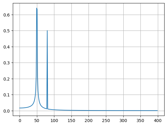
FFT Example: Sum of two Sines#
from scipy.fft import fft, fftfreq

# Number of sample points
N = 600
# sample spacing
T = 1.0 / 800.0
x = np.linspace(0.0, N * T, N, endpoint=False)
y = np.sin(50.0 * 2.0 * np.pi * x) + 0.5 * np.sin(80.0 * 2.0 * np.pi * x)
yf = fft(y)
xf = fftfreq(N, T)[: N // 2]
import matplotlib.pyplot as plt

plt.plot(xf, 2.0 / N * np.abs(yf[0 : N // 2]))
plt.grid()
plt.show()
FFT Helper Functions#
The function fftfreq returns the FFT sample frequency points.
f = [0, 1, ...,   n/2-1,     -n/2, ..., -1] / (d*n)   if n is even
f = [0, 1, ..., (n-1)/2, -(n-1)/2, ..., -1] / (d*n)   if n is odd
from scipy.fft import fftfreq

freq = fftfreq(8, 0.125)
freq
array([ 0., 1., 2., 3., -4., -3., -2., -1.])
The function fftshift allows swapping the lower and upper halves of a vector so that it becomes suitable for display. This shift the zero-frequency component to the center of the spectrum.
from scipy.fft import fftshift

x = np.arange(8)
print(fftshift(x))

freqs = np.fft.fftfreq(10, 0.1)
print(np.fft.fftshift(freqs))
[4 5 6 7 0 1 2 3]
[-5. -4. -3. -2. -1.  0.  1.  2.  3.  4.]
from scipy.fft import fft, fftfreq, fftshift
import matplotlib.pyplot as plt

# number of signal points
N = 400
# sample spacing
T = 1.0 / 800.0
x = np.linspace(0.0, N * T, N, endpoint=False)
y = np.exp(50.0 * 1.0j * 2.0 * np.pi * x) + 0.5 * np.exp(-80.0 * 1.0j * 2.0 * np.pi * x)
yf = fft(y)
xf = fftfreq(N, T)
xf = fftshift(xf)
yplot = fftshift(yf)

plt.plot(xf, 1.0 / N * np.abs(yplot))
plt.show()

Scipy has many other useful functions. If interested, you can look at the source documentation.