⏰ Late Assignments#
We expect that you will complete your assignments on time. However, we understand sometimes life gets in the way. What is most important is that you complete all of the assignments as it is essential for the learning process. Due to the size of the class and the use of automated grading technologies, we will not have the ability to make individual exceptions for late assignments. However, we will allow you to submit late assignments with a score deduction based on how late the submission is received.
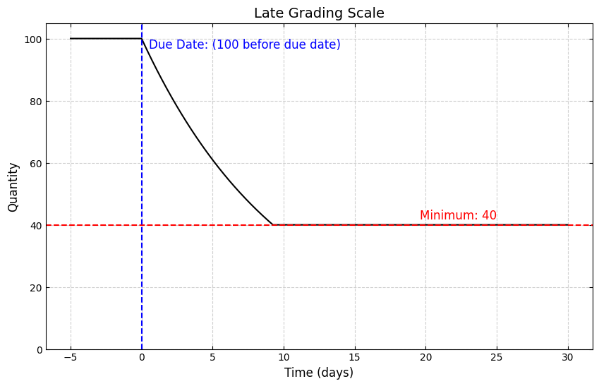
If submitted on time (before the due date), the assignment will receive your score weighted by 100% - full credit. After the due date, the score will decay exponentially to a minimum weighting of 40%, based on how late the submission is, measured in seconds past the due date.
The score weighting function is defined as:
Explanation of Substituted Values:#
\(Q_0 = 100\): Initial score before the due date.
\(Q_{\text{min}} = 40\): Minimum possible score for late submissions.
\(k = 6.88 \times 10^{-5}\): Decay constant.
\(t\): Time (in seconds) past the due date. Negative values of \(t\) indicate on-time submissions.
Show code cell source
import matplotlib.pyplot as plt
import numpy as np

# Parameters
Q0 = 100  # Initial quantity
Q_min = 40  # Minimum grade/quantity
k = 6.88e-5  # Decay constant per minute
time_in_seconds = np.linspace(
    -5 * 24 * 60 * 60, 30 * 24 * 60 * 60, 1000
)  # Time in seconds for 1 day before to 30 days after

# Exponential decay function with piecewise definition
Q = Q0 * np.exp(-k * time_in_seconds / 60)  # Convert seconds to minutes
Q = np.maximum(Q, Q_min)  # Apply floor condition
Q = np.minimum(Q, 100)  # Apply ceiling condition

# Plot
plt.figure(figsize=(10, 6))
plt.plot(
    time_in_seconds / (24 * 60 * 60),
    Q,
    label="Piecewise Exponential Decay",
    color="black",
)  # Convert seconds to days
plt.ylim(0, 105)
plt.title("Late Grading Scale", fontsize=14)
plt.xlabel("Time (days)", fontsize=12)
plt.ylabel("Quantity", fontsize=12)
plt.grid(True, linestyle="--", alpha=0.6)

# Horizontal and vertical lines with direct labels
plt.axhline(Q_min, color="red", linestyle="--")
plt.text(
    max(time_in_seconds) / (24 * 60 * 60) - 5,
    Q_min + 2,
    f"Minimum: {Q_min}",
    color="red",
    fontsize=12,
    ha="right",
)

plt.axvline(0, color="blue", linestyle="--")
plt.text(
    0.5,
    97,
    "Due Date: (100 before due date)",
    color="blue",
    fontsize=12,
    ha="left",
)

# Make ticks face inwards and on all 4 sides
plt.tick_params(axis="both", which="both", direction="in", top=True, right=True)

# Show plot
plt.show()