
📝 Symbolic Computation with SymPy#
“Solving Your Physics Homework the Easy Way!”

🤖 What is Symbolic Computation?#
Definition
Symbolic computation allows you to compute, manipulate, and simplify mathematical expressions exactly—without numerical approximations.
Think of it as Newton’s Calculus Notebook in code form.
Instead of approximating ( \(\sqrt{8} = 2.828\) ), SymPy simplifies it to ( \(2\sqrt{2}\) )—perfect for solving exact classical mechanics problems like trajectories or forces.
Historical Roots: Symbolic computation has its origins in Newtonian mechanics (17th century), where exact solutions were critical for describing planetary motion. 🌍
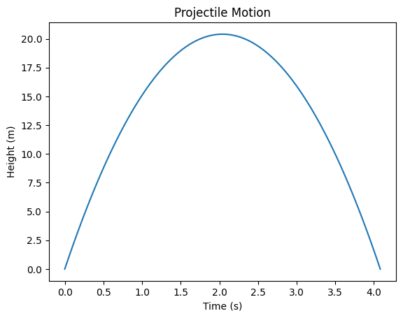
Example 1: Projectile Motion – Solving for Time#
Problem:#

Find the time ( \(t\) ) when a projectile hits the ground. The height equation is: $\( h(t) = v_0t - \frac{1}{2}gt^2 \)$
Variables:#
(\(h(t)\)): Height at time (\(t\))(\(m\)).
(\(v_0\)): Initial velocity (\(m/s\)).
(\(g\)): Acceleration due to gravity ((9.8 \(\text{m/s}^2\))).
(\(t\)): Time (\(s\)).
Code:#
from sympy import symbols, solve
from sympy import init_printing

init_printing()  # Enables the best option for your environment

v0, g, t = symbols("v0 g t")
h = v0 * t - (1 / 2) * g * t**2
time = solve(h, t)
time

Explanation:#
(\(t = 0\)): When the projectile is launched.
(\(t = \frac{2v_0}{g}\)): When the projectile hits the ground.
Visualization:#
import numpy as np
import matplotlib.pyplot as plt

v0 = 20  # Initial velocity in m/s
g = 9.8  # Gravity in m/s^2
t = np.linspace(0, 2 * v0 / g, 100)
h = v0 * t - 0.5 * g * t**2

plt.plot(t, h)
plt.title("Projectile Motion")
plt.xlabel("Time (s)")
plt.ylabel("Height (m)")
plt.show()
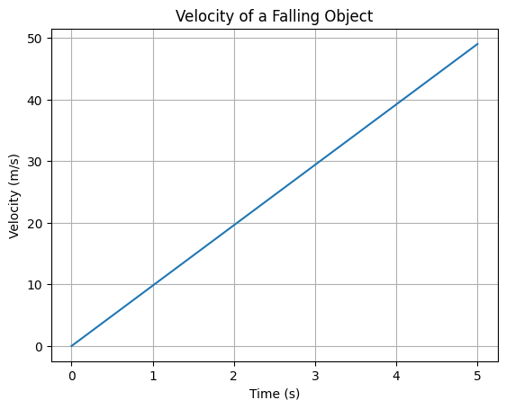
Example 2: Derivatives – Velocity from Position#
Problem:#
Derive the velocity equation from the position function of a falling object:
$\( s(t) = \frac{1}{2}gt^2\)$
Variables:#
(\(s(t)\)): Position (\(m\)).
(\(g\)): Gravity ((9.8 \(\text{m/s}^2)\)).
(\(t\)): Time (\(s\)).
Code:#
from sympy import diff

s, g, t = symbols("s g t")
s = (1 / 2) * g * t**2
v = diff(s, t)
v

Output:#
\(v(t) = g \cdot t\)
Visualization:#
g = 9.81  # Gravity in m/s^2
t = np.linspace(0, 5, 100)
v = g * t

plt.plot(t, v)
plt.title("Velocity of a Falling Object")
plt.xlabel("Time (s)")
plt.ylabel("Velocity (m/s)")
plt.grid()
plt.show()
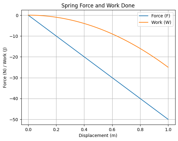
Example 3: Work Done by a Spring#

Problem:#
Calculate the work ( W ) done by a spring stretched from ( \(x = 0\) ) to ( \(x = 1\) ):
$\(F(x) = -kx \quad \text{and} \quad W = \int F(x) dx\)$
Variables:#
(\(F(x)\)): Force (\(N\)).
(\(k\)): Spring constant (\(\text{N/m}\)).
(\(x\)): Displacement (\(m\)).
Code:#
k, x = symbols("k x")
F = -k * x
W = F.integrate((x, 0, 1))
W

Output:#
Visualization:#
x = np.linspace(0, 1, 100)
k = 50  # Spring constant
F = -k * x
W = -0.5 * k * x**2

plt.plot(x, F, label="Force (F)")
plt.plot(x, W, label="Work (W)")
plt.title("Spring Force and Work Done")
plt.xlabel("Displacement (m)")
plt.ylabel("Force (N) / Work (J)")
plt.legend()
plt.grid()
plt.show()
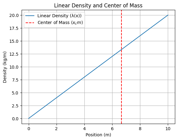
Example 4: Center of Mass#

Problem:#
Find the center of mass ( \(x_{cm}\) ) of a rod with length ( \(L\) ) and a linear density ( \(\lambda(x) = \lambda_0x\) ): $\(x_{cm} = \frac{\int_0^L x\lambda(x)dx}{\int_0^L \lambda(x)dx}\)$
Variables:#
( \(\lambda(x)\) ): Linear density (( \(\text{kg/m}\) )).
( \(L\) ): Length of the rod (\(m\)).
( \(x\) ): Position along the rod (\(m\)).
Code:#
from sympy import integrate

lambda0, L, x = symbols("lambda0 L x")
numerator = integrate(x * lambda0 * x, (x, 0, L))
denominator = integrate(lambda0 * x, (x, 0, L))
x_cm = numerator / denominator
x_cm

Output:#
\(x_{cm} = \frac{2L}{3}\)
Visualization:#
x = np.linspace(0, 10, 100)
lambda0 = 2  # Linear density constant
L = 10  # Length of rod
density = lambda0 * x

plt.plot(x, density, label="Linear Density (λ(x))")
plt.axvline(x=L * 2 / 3, color="red", linestyle="--", label="Center of Mass ($x_cm$)")
plt.title("Linear Density and Center of Mass")
plt.xlabel("Position (m)")
plt.ylabel("Density (kg/m)")
plt.legend()
plt.grid()
plt.show()
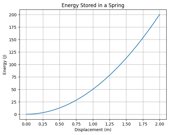
Example 5: Energy in a Spring System#

Problem:#
Calculate the total energy ( \(E\) ) stored in a spring stretched to ( \(x = a\) ):
\(E = \frac{1}{2}kx^2\)
Variables:#
( \(E\) ): Energy (\(J\)).
( \(k\) ): Spring constant (( \(\text{N/m}\) )).
( \(x\) ): Displacement (\(m\)).
Code:#
k, x = symbols("k x")
E = (1 / 2) * k * x**2
E

Output:#
Visualization:#
x = np.linspace(0, 2, 100)
k = 100  # Spring constant
E = 0.5 * k * x**2

plt.plot(x, E)
plt.title("Energy Stored in a Spring")
plt.xlabel("Displacement (m)")
plt.ylabel("Energy (J)")
plt.grid()
plt.show()
Why SymPy for Classical Mechanics?#
Exact Solutions: No approximations—ideal for forces, energies, and motion.
Visualization: Combine symbolic calculations with numerical plotting for deeper insights.
Free and Open Source: A perfect alternative to costly tools like Mathematica.
“With SymPy, solving Newtonian mechanics problems becomes exact and intuitive—just like Newton intended!” 🚀