📝 Overfitting

This might be a comfy bed for you, but I don’t know if your friend would like to sleep on it ☺️

• It is possible to get perfect accuracy on a test set but cannot conduct inference on a new problem

• The model is not generalizable

A model can classify types of apples but show it an orange and it is useless

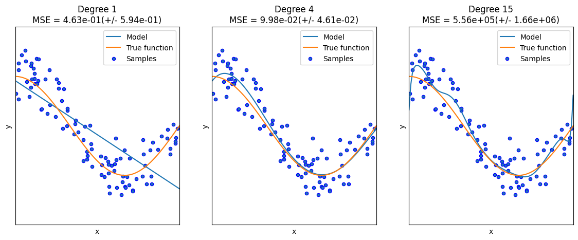
Overfitting Example with Polynomials

import numpy as np
import matplotlib.pyplot as plt
from sklearn.pipeline import Pipeline
from sklearn.preprocessing import PolynomialFeatures
from sklearn.linear_model import LinearRegression
from sklearn.model_selection import cross_val_score


# Defines the function
def true_fun(X):
    return np.cos(1.5 * np.pi * X)


# sets a random seed for consistent plotting
np.random.seed(0)

# sets the number of samples
n_samples = 100

# Sets the range in degrees
degrees = [1, 4, 15]

# adds some noise to the data
X = np.sort(np.random.rand(n_samples))
y = true_fun(X) + np.random.randn(n_samples) * 0.3

# does the plotting
plt.figure(figsize=(14, 5))

# Loops around the number of degrees selected
for i in range(len(degrees)):

    # makes the subplot
    ax = plt.subplot(1, len(degrees), i + 1)
    plt.setp(ax, xticks=(), yticks=())

    # creates the polynomial
    polynomial_features = PolynomialFeatures(degree=degrees[i], include_bias=False)

    # Least squares linear regression
    linear_regression = LinearRegression()

    # establishes a fitting pipeline
    pipeline = Pipeline(
        [
            ("polynomial_features", polynomial_features),
            ("linear_regression", linear_regression),
        ]
    )

    # does the fit
    pipeline.fit(X[:, np.newaxis], y)

    # Evaluate the models using crossvalidation
    scores = cross_val_score(
        pipeline, X[:, np.newaxis], y, scoring="neg_mean_squared_error", cv=10
    )

    # Defines a linear vector
    X_test = np.linspace(0, 1, 100)

    # plots the real model
    plt.plot(X_test, pipeline.predict(X_test[:, np.newaxis]), label="Model")
    plt.plot(X_test, true_fun(X_test), label="True function")

    # plots the generated data
    plt.scatter(X, y, edgecolor="b", s=20, label="Samples")

    # sets the axes format
    plt.xlabel("x")
    plt.ylabel("y")
    plt.xlim((0, 1))
    plt.ylim((-2, 2))
    plt.legend(loc="best")
    plt.title(
        "Degree {}\nMSE = {:.2e}(+/- {:.2e})".format(
            degrees[i], -scores.mean(), scores.std()
        )
    )