
📖 🧮 SymPy Calculus: Driving Engineering Solutions#
SymPy isn’t just for solving abstract math—it powers solutions for real-world engineering challenges, from ancient bridge designs to cutting-edge quantum tech. Let’s see how! 🌟
⚡ Derivatives: The Mathematics of Change#
Derivatives describe how things evolve, making them crucial for engineering design and analysis. SymPy handles everything from simple to multivariable derivatives.
Note
A derivative is a fancy way of saying “how fast something is changing at a specific moment.” Imagine you’re driving, and your speedometer says 60 mph—that’s your derivative, showing how quickly your position is changing over time. In math, it’s like measuring the steepness (slope) of a hill on a graph: flat ground means zero change, while a steep hill means big change. For example, if your function is \((y = x^2)\), the derivative is \((2x)\), which tells you how fast \((y)\) (your height) is growing as \((x)\) (your position) increases. It’s the ultimate “rate of change” detective! 🚗📈
Examples:#
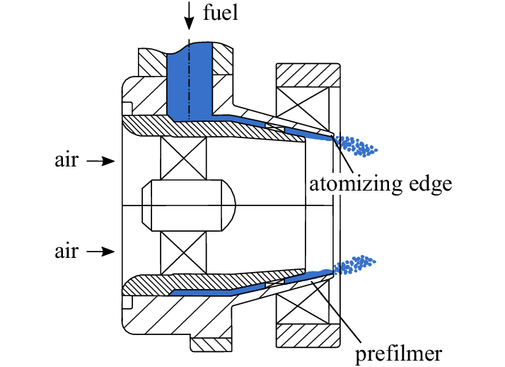
Fuel Atomizer Design: Optimizing the spray pattern in jet engines requires understanding the rate of change of liquid velocity:
from sympy import *

x, y, z, r = symbols("x y z r")

velocity = exp(-(x**2))
diff(velocity, x)
Seismology: Studying how stress waves propagate in Earth’s crust:
stress_wave = exp(-x * y * z)
diff(stress_wave, x, y, z)
18th-Century Cannonball Trajectories: The derivative of drag force was critical for modeling projectile motion:
drag_force = x**3 + 2 * x**2
diff(drag_force, x)
🔄 Integrals: Summing the Infinite#
Integrals are essential for finding areas, volumes, and even probabilistic outcomes. With SymPy, you can compute both definite and indefinite integrals easily.
Note
An integral is like finding the total stuff you’ve accumulated over time—whether it’s distance traveled, pizza eaten, or money earned. Imagine you’re driving, and your speedometer shows 60 mph; the integral tells you how far you’ve gone after driving for a while. On a graph, it’s like shading the area under a curve to figure out the total amount. For example, if your function is \((y = x^2)\), the integral gives you \((\frac{x^3}{3})\), which tells you how much “stuff” you’ve piled up as \((x)\) grows. It’s basically math’s way of keeping track of everything you’ve gathered! 🚗🛑📦
Examples:#
Thermal Management in Microchips: Calculate heat flux across a silicon wafer (area under a parabolic curve):
heat_flux = integrate(2 * x**2, (x, 0, 1))
heat_flux
Oil Reservoir Engineering: Modeling the volume of extracted oil using a radial integral:
integrate(2 * pi * r**2, (r, 0, 5))
18th-Century Tidal Energy: Early hydroelectric pioneers used integrals to calculate water flow potential:
integrate(exp(-x), (x, 0, oo))
🚦 Limits: Behavior at the Edges#
Limits help us understand system behaviors at extremes, such as in instability analysis or infinite load testing.
Note
A limit is like peeking at what happens when you get really close to a specific point. Imagine you’re driving, and you’re about to hit a wall; the limit tells you how close you can get without crashing. In math, it’s like seeing what happens to a function as you approach a certain value. For example, if your function is \((y = \frac{1}{x})\), the limit as \((x)\) approaches zero is infinity, showing that the function grows without bound as you get closer to zero. It’s like math’s way of predicting the future! 🚗🔍🔮
Examples:#
Supersonic Aircraft Design: Limiting behavior of air density at high altitudes:
Note
oo is a representation of the mathematical symbol for infinity.
air_density = limit(1 / x, x, oo)
Crystal Growth in Microgravity: Studying the behavior of concentration gradients as the crystal grows infinitely large:

concentration_gradient = x**2 / exp(x)
limit(concentration_gradient, x, oo)
Early Telecommunication Lines: Maxwell’s equations in 19th-century telegraph wires relied on limits to analyze signal decay:
signal = (cos(x) - 1) / x
limit(signal, x, 0)
🔍 Series Expansions: Simplifying the Complex#
Series expansions approximate complex behaviors, such as when studying chaotic or oscillatory systems.
Note
A series expansion is like taking a complicated function and breaking it into a simple recipe of smaller, easier-to-handle pieces. Imagine you’re making a pizza 🍕, and instead of looking at the whole thing, you think of it as layers: dough + sauce + cheese + toppings. Similarly, a series expansion rewrites a function as a sum of terms, like \((1 + x + x^2/2! + x^3/3! + \dots)\). Each term adds more detail, so the more terms you include, the closer you get to the real thing. It’s math’s way of saying, “Let’s build something big, one step at a time!” 🚀📜
Examples:#
Vibrations in Old Clock Towers: Modeling pendulum swings in tall clock mechanisms with Taylor series:

pendulum = exp(sin(x))
pendulum.series(x, 0, 4)
Aerodynamics of Helicopter Blades: Approximating airflow disturbances with polynomial expansions:
turbulence = exp(-x)
turbulence.series(x, 0, 6)
1700s Steam Engine Piston Analysis: Early engineers used series to predict small-scale pressure changes in pistons:
pressure = exp(x**2)
pressure.series(x, 0, 4)
🛠️ Finite Differences: For Real-World Data#
Finite differences estimate derivatives or integrals when functions are unknown—perfect for experimental data or simulations.
Note
Finite difference is like approximating a derivative by using simple math on a table of numbers. Imagine you’re tracking your car’s position at different times: 0m, 10m, 30m. Instead of using fancy calculus, you find the change in position divided by the change in time to estimate your speed. For example, if you go from 10m to 30m in 5 seconds, your speed is \(((30 - 10) / (5 - 0) = 4 \, \text{m/s})\). Finite differences work like this: they approximate rates of change by subtracting nearby values, perfect for computers or when exact formulas are too messy! 📊➖📈
Examples:#
Structural Health Monitoring: Use finite differences to detect cracks in aging bridges (measuring strain rates over discrete points):
# Define the symbolic variable
x = symbols("x")

# Define symbolic functions
f = Function("f")
g = Function("g")

# Perform symbolic differentiation
expression = f(x) * g(x)
result = diff(expression, x)

print("The derivative is:")
result
The derivative is:
Dust Accumulation in Space Telescopes: Use finite differences to study the rate of contamination over time:

dfdx = f(x).diff(x)
dfdx.as_finite_difference()
Medieval Siege Catapults: Engineers used early finite differences (pre-Newton!) to estimate projectile motion.
🌟 SymPy: An Engineer’s Swiss Army Knife#
SymPy transforms calculus from an abstract tool into a practical powerhouse. From optimizing 18th-century cannonballs to designing 21st-century silicon chips, it bridges historical ingenuity and modern innovation. Ready to explore the possibilities? 🚀✨