🧪 🔩⚙️💪 Designing Composites with Optimal Mechanical Properties

# You must make sure to run all cells in sequence using shift + enter or you might encounter errors
from pykubegrader.initialize import initialize_assignment

responses = initialize_assignment("1_lab_composite", "week_3", "lab", assignment_points = 41.0, assignment_tag = 'week3-lab')

# Initialize Otter
import otter
grader = otter.Notebook("1_lab_composite.ipynb")

🧪 🔩⚙️💪 Designing Composites with Optimal Mechanical Properties#

Introduction#

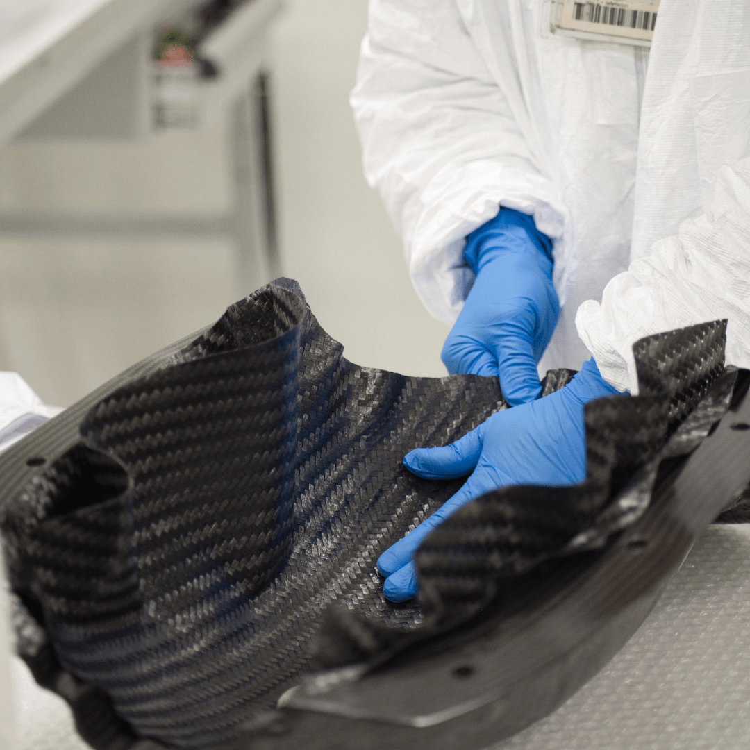
Composite materials are advanced materials engineered by combining two or more distinct constituent materials, each with significantly different physical or chemical properties. The resulting composite exhibits unique characteristics that differ from those of its individual components, while the constituents remain separate and distinct within the final structure.

The objective of this lab is to leverage NumPy to develop a robust system for calculating the properties of a composite material based on the properties of its individual components, their volume fractions, and the orientation of fibers. This capability is crucial for designing high-performance materials and structures. For example, carbon fiber composites are widely used in aerospace applications due to their exceptional strength-to-weight ratio. Accurate prediction of the properties of these materials is vital to ensure they meet application-specific requirements and to design materials with tailored properties along different axes.

Goals:#

You want to compute the effective stiffness of a 2D composite (plane stress) reinforced by short fibers (or platelets) whose orientations are not uniform—instead, they follow some anisotropic orientation distribution. Each filler phase has local stiffness $\mathbf{Q}_\text{local}$ in its principal axes, and you also know the matrix stiffness. Your goal is to:

Define the 2D plane-stress stiffness matrix $\mathbf{Q}_\text{local}$ for the filler in its local coordinate system (aligned with principal directions).
Rotate that local stiffness into the global coordinates for each orientation $\theta$ the filler may have, using a transformation matrix $\mathbf{T}(\theta)$.
Combine these rotated filler stiffness matrices, weighted by their orientation distribution (i.e., the fraction of fibers oriented at each $\theta$), and then add the matrix contribution to get the overall effective stiffness of the composite.

Your tasks are to Write a Python/NumPy script that:#

Builds a local filler stiffness matrix $\mathbf{Q}_\text{local}$.
Implements rotation of $\mathbf{Q}_\text{local}$ to $\mathbf{\bar{Q}}(\theta)$ for a given $\theta$.
Summation or integration of $\mathbf{\bar{Q}}(\theta)$ across the anisotropic distribution to get $\mathbf{Q}_\text{filler,eff}$.
Combines the filler result with matrix stiffness to obtain the final $\mathbf{Q}_\text{eff}$.

Don’t Worry you are not expected to know the math required to solve this problem, we will guide you through the process, and explain the math behind the solution as we go along.

Part 1: Matrix Stiffness#

First, we want to define the 2D plane stiffness matrix. The stiffness matrix $\mathbf{Q}$ provides the stiffness of the material along all axis in the material coordinate system. The stiffness matrix is a 3x3 matrix for 2D plane stress problems.

\[\begin{split} \mathbf{Q}_\text{local} = \begin{bmatrix} Q_{11} & Q_{12} & 0 \\ Q_{12} & Q_{22} & 0 \\ 0 & 0 & G_{12} \end{bmatrix}. \end{split}\]

$Q_{11}$:
This is the stiffness in the 1-direction (typically aligned with the fiber’s principal axis). It quantifies the material’s resistance to normal strain along the 1-direction when subjected to normal stress in the same direction.
$Q_{22}$:
This is the stiffness in the 2-direction (perpendicular to the 1-direction in the plane). It quantifies the material’s resistance to normal strain along the 2-direction when subjected to normal stress in the same direction.
$Q_{12}$:
This represents the coupling stiffness between the 1- and 2-directions. It arises from the material’s anisotropy, where normal stress in one direction may cause strain in the perpendicular direction.
$G_{12}$:
This is the in-plane shear modulus, which quantifies the material’s resistance to in-plane shear deformation. It is a measure of the stiffness associated with shearing action in the plane of the composite.
0 entries:
The zero entries indicate that there is no coupling between shear deformation and normal stresses (in-plane shear stresses do not cause normal strains and vice versa) in the principal axes. This is a characteristic of the orthotropic behavior assumed in this matrix.

In this case we will assume that the matrix stiffness is isotropic, meaning that the stiffness is the same in all directions.

Make sure you do not hardcode the values of the stiffness matrix, instead use the variables provided in the code cell below

Python Implementation:#

We will begin by implementing the local filler stiffness matrix $\mathbf{Q}_\text{local}$ in Python using NumPy. To achieve this, we define a function local_stiffness_matrix that takes the following parameters as input:

Elastic moduli: $E_1$ and $E_2$,
Poisson’s ratio: $\nu_{12}$,
Shear modulus: $G_{12}$.

The function will return the local stiffness matrix $\mathbf{Q}_\text{local}$. We have provided the scaffolding for the function, and you need to fill in the missing code.

compute the Poisson’s ratio in the transverse direction, denoted as $\nu_{21}$ to the variable v21, based on the given Poisson’s ratio in the longitudinal direction ($\nu_{12}$) and the elastic moduli ($E_1$ and $E_2$), using the formula: $$ \nu_{21} = \frac{E_2}{E_1} \cdot \nu_{12} $$
Compute the denominator factor denom which is used to compute the stiffness matrix components, using the formula: $$ denom = 1 - \nu_{12} \cdot \nu_{21} $$
Compute the stiffness matrix components $Q_{11}$, $Q_{22}$, and $Q_{12}$ and assign them to the variables Q11, Q22, and Q12 respectively using the formulas: $$ Q_{11} = \frac{E_1}{1 - \nu_{12} \cdot \nu_{21}} $$ Q_{22} = \frac{E_2}{1 - \nu_{12} \cdot \nu_{21}} $$ Q_{12} = \frac{\nu_{12} \cdot E_2}{1 - \nu_{12} \cdot \nu_{21}} $$
Construct the local stiffness matrix as a 2D NumPy array Q using the computed stiffness matrix components $Q_{11}$, $Q_{22}$, and $Q_{12}$, per the matrix definition provided:

\[\begin{split} \mathbf{Q}_\text{local} = \begin{bmatrix} Q_{11} & Q_{12} & 0 \\ Q_{12} & Q_{22} & 0 \\ 0 & 0 & G_{12} \end{bmatrix}. \end{split}\]

in python you can use the np.array function to create a 2D array. The syntax should look like this:

Q = np.array([[Q11, Q12, 0],
              [Q12, Q22, 0],
              [0, 0, G12]])

Compute the matrix stiffness tensor:

Use the local_stiffness_orthotropic function to compute the local stiffness matrix for the filler phase with the following properties:

Elastic modulus in the 1-direction: $E_1 = E_2 = 2$ GPa
Poisson’s ratio in the 1-direction: $\nu_{12} = 0.33$
Shear modulus: $G_{12} = 0.8$ GPa

Assign this to the variable Q_matrix.

import numpy as np


def local_stiffness_orthotropic(E1, E2, v12, G12, otter=False):

    # 1. Compute the transverse Poisson's ratio
    ...

    # 2. Compute the denominator of the stiffness matrix Q
    ...

    # 3. Compute the stiffness matrix Q
    ...

    # 4. Assemble the stiffness matrix Q
    ...
    
    # DO NOT MODIFY the following code
    if otter:
        return Q, E1, E2, v12, G12, v21, denom, Q11, Q22, Q12
    return Q


# This is used to test the function
Q_matrix = local_stiffness_orthotropic(2, 2, 0.33, 0.8)

grader.check("local_stiffness_orthorhombic")

Part 2: Rotation Matrix to Transform from Local to Global Coordinates#

Context#

In 2D plane stress problems, we typically work with stress components ($\sigma_x, \sigma_y, \tau_{xy}$) or strain components ($\epsilon_x, \epsilon_y, \gamma_{xy}$) defined in the local or global coordinate system. These components can be transformed between coordinate systems using a transformation matrix ($\mathbf{T}(\theta)$), where $\theta$ represents the angle of rotation between the local and global axes.

The transformation matrix ($\mathbf{T}(\theta)$) is derived based on trigonometric relationships in the rotated coordinate system. The components of the transformation matrix account for how normal and shear stresses/strains change under rotation.

For engineering applications like composite materials or anisotropic elasticity, it is often necessary to compute the stiffness matrix ($\mathbf{\bar{Q}}$) in the global coordinate system from the stiffness matrix ($\mathbf{Q}_\text{local}$) in the local coordinate system. This transformation involves both the transformation matrix and its transpose/inverse, as shown below.

Stress/Strain Representation in Plane Stress#

\[ \text{Stress components: } \sigma_x, \sigma_y, \tau_{xy} \]

\[ \text{Strain components: } \epsilon_x, \epsilon_y, \gamma_{xy} \]

Transformation Matrix (3×3)#

\[\begin{split} \mathbf{T}(\theta) = \begin{bmatrix} \cos^2\theta & \sin^2\theta & 2\sin\theta \cos\theta \\ \sin^2\theta & \cos^2\theta & -2\sin\theta \cos\theta \\ -\sin\theta \cos\theta & \sin\theta \cos\theta & \cos^2\theta - \sin^2\theta \end{bmatrix}. \end{split}\]

Stiffness Transformation#

\[ \mathbf{\bar{Q}}(\theta) = \mathbf{T}^{-1}(\theta) \; \mathbf{Q}_\text{local} \; \mathbf{T}^{-T}(\theta) \]

where:

$ \mathbf{\bar{Q}}(\theta) \text{ is the global stiffness matrix.} $

$ \mathbf{Q}_\text{local} \text{ is the stiffness matrix in the local coordinate system.} $

$ \mathbf{T}(\theta) \text{ is the transformation matrix.} $

$ \mathbf{T}^{-1} \text{ and } \mathbf{T}^{-T} \text{ are the inverse and transpose-inverse of } \mathbf{T}(\theta), \text{ respectively.} $

Python Implementation:#

Part 2.1: Rotation Matrix#

We will implement a function rotation_matrix that computes the transformation matrix $\mathbf{T}(\theta)$ for a given angle $\theta$. The function will take the angle $\theta$ as input and return the transformation matrix $\mathbf{T}(\theta)$.

Compute the trigonometric functions $\sin\theta$ and $\cos\theta$ using NumPy’s sin and cos functions, respectively. Assign the results to the variables sin_theta and cos_theta.
Construct the transformation matrix $\mathbf{T}(\theta)$ as a 2D NumPy array T using the computed trigonometric functions $\sin\theta$ and $\cos\theta$, per the matrix definition provided:

\[\begin{split} \mathbf{T}(\theta) = \begin{bmatrix} \cos^2\theta & \sin^2\theta & 2\sin\theta \cos\theta \\ \sin^2\theta & \cos^2\theta & -2\sin\theta \cos\theta \\ -\sin\theta \cos\theta & \sin\theta \cos\theta & \cos^2\theta - \sin^2\theta \end{bmatrix}. \end{split}\]

recall:

\[ \sin^2 \theta = (\sin \theta)^2 \quad \text{and} \quad \cos^2 \theta = (\cos \theta)^2 \]

def transformation_matrix_2D(theta, otter=False):
    """
    Build the 3x3 transformation matrix for plane-stress (sigma_x, sigma_y, tau_xy).
    """
    # 1. Compute the cosine and sine of the angle theta
    ...

    # 2. Build the transformation matrix
    ...

    if otter:
        return T, cos_theta, sin_theta
    return T

grader.check("transformation-matrix-2d")

Part 2.2: Transformation of Stiffness Matrix#

Next, we will implement a function transform_stiffness that computes the transformed stiffness matrix $\mathbf{\bar{Q}}(\theta)$ in the global coordinate system for a given local stiffness matrix $\mathbf{Q}_\text{local}$ and angle $\theta$. The function will take the local stiffness matrix $\mathbf{Q}_\text{local}$ and angle $\theta$ as inputs and return the transformed stiffness matrix $\mathbf{\bar{Q}}(\theta)$.

Compute the transformation matrix $\mathbf{T}(\theta)$ using the transformation_matrix_2D function with the input angle $\theta$. To do this, call the transformation_matrix_2D function with the input angle $\theta$ and assign the result to the variable T. You can call the function you wrote just like any function you import from a library.
Compute the inverse of the transformation matrix $\mathbf{T}^{-1}(\theta)$ using NumPy’s linalg.inv function. Assign the result to the variable T_inv.
Compute the transpose-inverse of the transformation matrix $\mathbf{T}^{-T}(\theta)$ using NumPy’s transpose built-in method. This can be easily done using the <2D Numpy Array>.T method. Assign the result to the variable T_inv_transpose.
Compute the transformed stiffness matrix $\mathbf{\bar{Q}}(\theta)$ using the formula provided:

\[\mathbf{\bar{Q}}(\theta) = \mathbf{T}^{-1}(\theta) \; \mathbf{Q}_\text{local} \; \mathbf{T}^{-T}(\theta)\]

Note: This is a matrix multiplication operation, and you can use the @ operator for matrix multiplication in NumPy. If you were to us the * operator, it would perform element-wise multiplication.

Note

Elementwise Multiplication: Each corresponding element of two matrices (or arrays) is multiplied independently. This operation requires matrices of the same shape and results in a matrix of the same dimensions, where each element is the product of the corresponding elements.

For example:

\[\begin{split} \begin{bmatrix} a & b \\ c & d \end{bmatrix} \odot \begin{bmatrix} e & f \\ g & h \end{bmatrix} = \begin{bmatrix} a \cdot e & b \cdot f \\ c \cdot g & d \cdot h \end{bmatrix} \end{split}\]

Matrix Multiplication: This follows the linear algebra rules for multiplying matrices. The elements of the resulting matrix are computed as the dot product of rows from the first matrix with columns from the second. For example:

\[\begin{split} \begin{bmatrix} a & b \\ c & d \end{bmatrix} \cdot \begin{bmatrix} e & f \\ g & h \end{bmatrix} = \begin{bmatrix} a \cdot e + b \cdot g & a \cdot f + b \cdot h \\ c \cdot e + d \cdot g & c \cdot f + d \cdot h \end{bmatrix} \end{split}\]

Key Difference: Elementwise multiplication is straightforward and independent for each element, while matrix multiplication involves summing products across rows and columns, capturing relationships between elements.

def transform_stiffness(Q_local, theta, otter=False):
    """
    Transform Q_local into global coords by angle theta.
    Q_bar = T_inv * Q_local * T_inv^T
    """
    # 1. Compute the transformation matrix T
    ...

    # 2. Compute the inverse of the transformation matrix T
    ...

    # 3. Compute the transpose of the inverse of the transformation matrix T
    ...

    # 4. Compute the transformed stiffness matrix Q_bar, remember to use the @ operator for matrix multiplication
    ...

    # Do not change the code below this line
    if otter:
        return T, T_inv, T_inv_transpose, Q_bar
    else:
        return Q_bar

grader.check("transform-stiffness")

Part 3: Effective Stiffness of Anisotropic Filler Distribution#

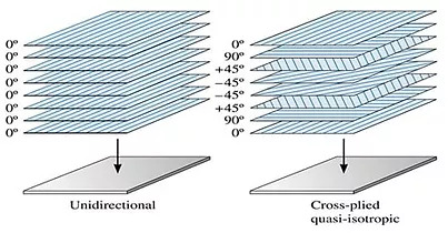
Generally, composite materials are designed with a specific orientation distribution of the filler phase to achieve desired mechanical properties. In this context, we will consider an anisotropic distribution of filler orientations in the composite material. The filler phase is assumed to have a local stiffness matrix $\mathbf{Q}_\text{local}$ in its principal axes, and the orientation distribution is characterized by the volume fraction of fibers $\phi_i$ oriented at each angle $\theta$. You can compute the effective stiffness of the composite material by computing the sum over all orientations:

\[ \mathbf{Q}_\text{filler}^\text{(eff)} = \sum_{i=1}^{n} \phi_i \, \mathbf{\bar{Q}}(\theta_i), \quad \text{where} \quad \mathbf{\bar{Q}}(\theta_i) = \text{transform\_stiffness}(\mathbf{Q}_\text{local}, \theta_i). \]

Python Implementation:#

initialize a 3 by 3 zero array Q_bar using the np.zeros function. This array will store the sum of the transformed stiffness matrices for each orientation.
Inside the loop convert the angle_deg to radians using the np.radians function and assign it to the variable theta_rad.
Compute the transformed stiffness matrix transformed_stiffness_matrix using the transform_stiffness function with the local stiffness matrix Q_local and the angle theta_rad.
Use the add assignment operator += to add the transformed_stiffness_matrix to the Q_bar array, weighted by the volume fraction phi_i.
Test this code by computing the effective stiffness matrix Q_filler_eff for following information.

5.1 Local Stiffness Matrix:

Compute the local stiffness matrix Q_local using the local_stiffness_orthotropic function with the given elastic moduli and shear modulus.

$E_1$ = 100 GPa $E_2$ = 10 GPa $\nu_{12}$ = 0.3
$G_{12}$ = 5 GPa

5.2 Filler Orientations and Volume Fractions: Make the following lists for the angles and volume fractions.

Angles - [0, 30, 60, 90] Volume Fractions - [0.12, 0.03, 0.02, 0.03]

To do this, make lists angles_deg and volume fractions phis for the angles and volume fractions, respectively.

5.3 Compute the effective filler stiffness Compute the effective filler stiffness by calling the compute_filler_stiffness function with the local stiffness matrix Q_local, angles in degrees angles_deg, and volume fractions phis as inputs. Assign the result to the variable Q_filler_eff.

def compute_filler_stiffness(Q_local, angles_deg, phis):
    """
    Compute the stiffness matrix for a laminate with given fiber angles and volume fractions.
    """
    # 1. Initialize the stiffness matrix
    ...

    # Do not modify this line of code, this code will iterate over the list of angles and phis one at a time
    # make sure that your code is tab indented inside the for loop
    for angle_deg, phi_i in zip(angles_deg, phis):

        # 2. Compute the angle in radians
        theta_rad = ...

        # 3. Compute the transformed stiffness matrix Q_bar
        transformed_stiffness_matrix = ...

        # 4. Update the global stiffness matrix Q_bar using the transformed stiffness matrix and the volume fraction
        ...

    # Do not change the code below this line
    return Q_bar


# 5.1 Compute the local stiffness matrix
...

# 5.2 Assign the list of fiber angles and volume fractions
...

# 5.3 Compute the global stiffness matrix
...

grader.check("composite-filler-stiffness")

Part 4: Effective Stiffness of Composite Material#

Now we need to add the mechanical properties of the matrix to determine the ensemble properties of the composite material. The effective stiffness matrix $\mathbf{Q}_\text{eff}$ of the composite material can be computed by adding the stiffness matrix of the matrix phase $\mathbf{Q}_\text{matrix}$ to the effective stiffness matrix of the filler phase $\mathbf{Q}_\text{filler}^\text{(eff)}$ weighted by their effective volume fractions.

Python Implementation:

Compute the fraction of the total composite composed of filler by taking the sum of the volume fractions phis and assign it to the variable f_filler. You should use the np.sum function to compute the sum of the volume fractions.
compute the effective stiffness matrix Q_eff by adding the matrix stiffness Q_matrix to the effective filler stiffness Q_bar weighted by the fraction of filler f_filler. The formula for computing the effective stiffness matrix is given by:

\[\mathbf{Q}_\text{eff} = (1 - f_\text{filler}) \cdot \mathbf{Q}_\text{matrix} + f_\text{filler} * \mathbf{Q}_\text{filler eff}\]

# Combine with matrix

# Compute the sum of the volume fractions
...

# Compute the effective stiffness matrix
...

# We have provided the code to print the results for you
print("Local Filler Q:\n", Q_local, "\n")
print("Matrix Q:\n", Q_matrix, "\n")
print("Effective Filler Q:\n", Q_filler_eff, "\n")
print("Overall Effective Q:\n", Q_eff)

grader.check("effective_stiffness_composite")

Visualization#

We have provided some visualizations to help you understand your results. You can run the code cell below to visualize the local stiffness matrix, the transformed stiffness matrix for different orientations, and the effective stiffness matrix of the composite material.

from composite_viz import *

# polar plot of stiffness vs orientation
plot_stiffness_polar(transform_stiffness, Q_local)

# Volume fraction for different fiber orientations
plot_volume_fractions(angles_deg, phis)

# Stiffness matrix
plot_stiffness_matrix(Q_eff, title="Effective Stiffness Matrix")

# Stiffness vs orientation linear
plot_stiffness_line(transform_stiffness, Q_local)

Submitting Assignment#

Please run the following block of code using shift + enter to submit your assignment, you should see your score.

from pykubegrader.submit.submit_assignment import submit_assignment

submit_assignment("week3-lab", "1_lab_composite")

🧪 🔩⚙️💪 Designing Composites with Optimal Mechanical Properties

Contents

🧪 🔩⚙️💪 Designing Composites with Optimal Mechanical Properties#

Introduction#

Goals:#

Your tasks are to Write a Python/NumPy script that:#

Part 1: Matrix Stiffness#

Python Implementation:#

Part 2: Rotation Matrix to Transform from Local to Global Coordinates#

Context#

Stress/Strain Representation in Plane Stress#

Transformation Matrix (3×3)#

Stiffness Transformation#

Python Implementation:#

Part 2.1: Rotation Matrix#

Part 2.2: Transformation of Stiffness Matrix#

Part 3: Effective Stiffness of Anisotropic Filler Distribution#

Python Implementation:#

Part 4: Effective Stiffness of Composite Material#

Visualization#

Submitting Assignment#