
📖 🧩 Solvers in SymPy: Cracking the Code of Engineering Problems#

From ancient bridge stress tests to quantum computing algorithms, solving equations has always been at the heart of engineering. SymPy’s solvers take this legacy into the digital age! Let’s explore. 🚀
✨ Equations: The Basics#
Equations in SymPy are handled with Eq or, even better, you can just assume = 0 for simplicity:
from sympy import *

x, y, z = symbols("x y z")

Eq(x**2 - 1, x)
💡 Historical Insight: Solving quadratic equations dates back to Babylon (~2000 BCE), where engineers used it for irrigation canal designs! 🌾
⚡ Algebraic Solvers#
solveset: The Workhorse#
SymPy’s solveset tackles algebraic equations with ease:
Crack Riddler’s Codes (Modular Arithmetic): Solve periodic equations in wave encryption:
Tip
Many solutions to expressions can contain real and imaginary solutions. Use domain to filter them.
solveset(sin(x) - 1, x, domain=S.Reals)
Oil Refinery Pipeline Optimization: Solve systems of equations to optimize flow in pipelines:
linsolve([x + y + z - 1, x + y + 2 * z - 3], (x, y, z))
💡 Obscure Use: 18th-century mining engineers used algebraic systems to calculate water drainage paths in complex mines. 🪨
🔄 Nonlinear Systems with nonlinsolve#
SymPy excels at solving nonlinear equations, even those with real and complex solutions:
Note
Non-linear systems of equations are like trying to solve a puzzle where the rules don’t follow straight lines. Instead of easy, predictable relationships (like \((x + y = 10)\)), you get curvy, messy ones (like \((x^2 + y^2 = 25)\), a circle). These systems involve equations with squares, cubes, or other funky stuff that make them bend, twist, or loop. Solving them is like figuring out where all the curves and loops meet—it’s trickier than straight-line math, but it’s how we handle real-world chaos, like predicting weather or designing rocket trajectories! 🌪️🚀📐
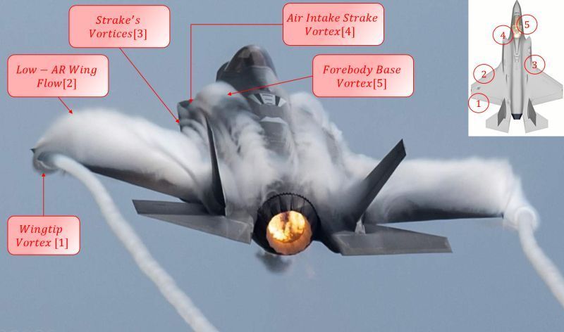
Vortex Behavior in Jet Engines: Solve flow equations with nonlinear dependencies:
nonlinsolve([x * y - 1, x - 2], [x, y]) # Output: {(2, 1/2)}
Acoustic Resonance in Concert Halls: Modeling sound wave interference:
nonlinsolve([x**2 + 1, y**2 + 1], [x, y])
💡 Historical Example: Early radio engineers solved nonlinear equations to tune vacuum tubes for clearer signals. 📻
🌊 Differential Equations with dsolve#
SymPy simplifies differential equations, critical for dynamic systems like vibrations, fluid flows, and control systems.
Note
Differential equations are like math’s way of describing how things change over time. Instead of just finding the answer, you’re solving for a rule about how something evolves—like how fast a car speeds up, how a virus spreads, or how coffee cools down. They involve derivatives (rates of change), so instead of saying \((y = 3x + 2)\), it’s more like, “How does \((y)\) change if it depends on \((x)\)?” For example, if you’re pouring water into a tank, a differential equation tells you how the water level rises as time passes. It’s the ultimate tool for modeling anything dynamic! 🚗📈🌊
Designing Ship Stabilizers: Model damping effects to counter ocean waves:

f = Function("f")

diffeq = Eq(f(x).diff(x, x) - 2 * f(x).diff(x) + f(x), sin(x))
dsolve(diffeq, f(x))
18th-Century Clock Escapements: Engineers modeled pendulum damping to design accurate clocks. 🕰️
🔍 Specialized Tools#
Roots with Multiplicity#
Note
Roots with multiplicity are like special “sticky” roots that affect how systems behave, which is super important in engineering. For example, in \(( (x - 2)^2 = 0 )\), the root \((x = 2)\) has multiplicity 2, meaning the graph just touches the x-axis at that point but doesn’t cross it. Why does this matter? In engineering, systems modeled by equations often depend on these roots. If a root has higher multiplicity, it changes the system’s stability or response. For instance, in vibrations or control systems, repeated roots can mean slower damping or lingering oscillations. Essentially, roots with multiplicity are like hidden clues that tell engineers how their designs will behave under stress or dynamic conditions! 🏗️📊⚙️

Find roots and their multiplicities with roots:
roots(x**3 - 6 * x**2 + 9 * x, x) # Output: {0: 1, 3: 2}
{3: 2, 0: 1}
💡 Example: Calculating shaft resonance frequencies in early wind turbines relied on understanding root multiplicities.
Lambert W for Transcendental#
Note
The Lambert W function is like a magical math tool for solving tricky equations where the variable is stuck in both the base and the exponent—a classic problem with transcendental equations. For example, if you have something like \(( x e^x = 5 )\), there’s no way to solve it using regular algebra. This is where the Lambert W function comes in! It “unsticks” the variable by essentially reversing \(( y = x e^x )\), giving \(( x = W(y))\).
Why does this matter for engineering? Many real-world problems involve transcendental equations—like modeling diode currents in electronics, finding growth rates in population models, or solving time constants in heat transfer. The Lambert W function simplifies these problems into something solvable, making it an indispensable tool in areas like circuit design, control systems, and thermodynamics. It’s like a Swiss army knife for dealing with equations that don’t play by algebra’s rules! 🔧📈✨
Solve tricky equations like x * exp(x) = 1:
solve(x * exp(x) - 1, x) # Output: [W(1)]
[LambertW(1)]
💡 Obscure Use: Hey Chemical Engineers, Lambert W functions helped chemists model reaction rates in high-pressure vessels during WWII. 🧪

🎯 Why SymPy Solvers Matter#
From ancient mine drainage to modern cryptography, SymPy’s solvers bridge the gap between math and engineering innovation. Whether it’s cracking nonlinear systems or modeling acoustic resonance, SymPy gives you the tools to conquer complex problems. Ready to solve? 🧮✨