📝 Monte Carlo in a Circle ◯

Is anything particularly interesting visualized if we randomly distribute points in a 2 dimensional, -1 by 1 grid on which is plotted a circle of radius 1 centered at (0,0)?

Monte Carlo simulations are a class of computational algorithms that rely on repeated random sampling to obtain numerical results. They are often used to model phenomena with significant uncertainty in inputs, such as the calculation of risk in business or the simulation of physical and mathematical systems. The basic idea is to use random numbers to simulate the behavior of a complex system, and then use the results to make predictions about the system’s behavior.

Import required packages

We will need packages to handle stats and visualization.

from IPython.display import display, clear_output
import matplotlib.pyplot as plt
import numpy as np
import random
import math
import time

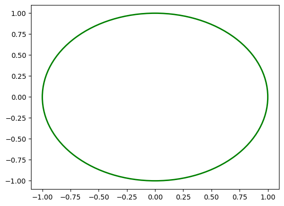
Plot Circle

Plot a circle of radius 1, centered at (0,0)

#Initialize plot 
fig, ax = plt.subplots()

#Set limits of visualization
ax.set_xlim(-1.1, 1.1)
ax.set_ylim(-1.1, 1.1)

#Place circle on plot 
circle = plt.Circle((0, 0), 1, fill=False, color='green', linewidth=2)
ax.add_artist(circle)

<matplotlib.patches.Circle at 0x7f93f5466e50>

Generate Data

#Initialize variables 
num_samples = 1000
points_inside_circle = 0
x_data, y_data = [], []

#Loop through desired sample to generate values for x and y based on uniform distribution 
for i in range(num_samples):
        x = random.uniform(-1, 1)
        y = random.uniform(-1, 1)
        x_data.append(x)
        y_data.append(y)
        distance = math.sqrt(x**2 + y**2)
        if distance <= 1:
                points_inside_circle += 1 

Plot data

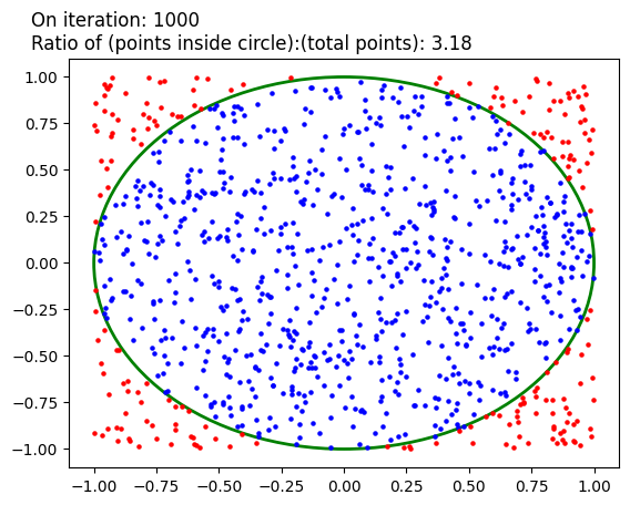
What is the ratio of points inside the circle vs. total points?

#Initialize plots for data inside circle and outside circle with different colors  
inside_scat = ax.scatter([], [], color='blue', s=5)
outside_scat = ax.scatter([], [], color='red', s=5) 

#Initialize variables to be populated with data for points inside vs outside circle
inside_x, inside_y = [], []
outside_x, outside_y = [], []
points_inside = 0

#Initialize text location
info_text = ax.text(-1.25, 1.15, "", fontsize=12, color="black")

#Loop through samples to populate inside/outside x and y points 
for i in range(num_samples):
        #if a point is inside the circle, add it the appropriate list 
        if (x_data[i])**2 + (y_data[i])**2 <= 1:
            inside_x.append(x_data[i])
            inside_y.append(y_data[i])
            points_inside += 1
        #otherwise, add it to the other list
        else:
            outside_x.append(x_data[i])
            outside_y.append(y_data[i])

        #combine and formatt both sets of data 
        offsets_in = np.array(list(zip(inside_x, inside_y)))
        offsets_out = np.array(list(zip(outside_x, outside_y)))

        #make sure that both sets of data are the correct shape, even if they are empty
        if offsets_in.ndim != 2:
            offsets_in = np.empty((0, 2))
        if offsets_out.ndim != 2:
            offsets_out = np.empty((0, 2))
       
        #add data to figure 
        inside_scat.set_offsets(offsets_in)
        outside_scat.set_offsets(offsets_out)


        total_points = len(inside_x) + len(outside_x)
        if total_points > 0:
            ratio_current = 4 * (len(inside_x) / total_points)
        else:
            ratio_current = 0.0
        info_text.set_text(
        f"On iteration: {i+1}\n"
        f"Ratio of (points inside circle):(total points): {ratio_current:.2f}"    
        )
        
        #animate addition of new points 
        clear_output(wait=True)
        display(fig)
        time.sleep(0.001)