🔍 Unsupervised Learning with Scikit-learn: Discovering Hidden Patterns 🎲

Imagine you’re an engineer managing a factory that produces thousands of parts daily. You don’t know the exact categories or defects, but you notice some parts look similar while others are completely different. 🤔

Wouldn’t it be amazing if you could group these parts automatically, without any predefined labels? Welcome to the magical world of Unsupervised Learning! 🎉

🤔 What is Unsupervised Learning?

Unsupervised Learning is like exploring a new city without a map:

• You observe everything around you.

• You group similar things together (like neighborhoods or landmarks).

• You discover patterns without any prior knowledge or labels.

🧠 In Simple Words:

Unsupervised Learning = Finding Patterns in Unlabeled Data

In engineering terms:

• You have lots of sensor data but no labels.

• You want to find patterns, anomalies, or group similar items.

• Goal: To organize and understand the data without supervision.

🔑 Key Types of Unsupervised Learning

1. Clustering 🎯

• Definition: Grouping data points that are similar to each other.

• Example:

  • Grouping customers based on buying behavior.

  • In manufacturing: Clustering defective parts based on dimensions and texture.

2. Dimensionality Reduction 🔻

• Definition: Reducing the number of features while retaining important information.

• Example:

  • Simplifying a complex dataset for visualization.

  • In engineering: Reducing sensor data dimensions for fault detection.

3. Anomaly Detection 🚨

• Definition: Identifying rare or unusual data points.

• Example:

  • Detecting fraudulent transactions.

  • In engineering: Identifying faulty sensors or equipment failures.

🧑‍🔧 Engineering Examples

⚙️ Example 1: Clustering Defective Parts

Imagine a factory producing bolts with different dimensions.

• Goal: Group the bolts into categories like “Normal”, “Too Long”, “Too Short”, “Too Thick”, or “Too Thin.”

• Approach: Use Clustering to discover natural groupings without predefined labels.

⚙️ Example 2: Anomaly Detection in Machine Health

In predictive maintenance, you monitor sensor data from machines.

• Goal: Detect anomalies to predict potential breakdowns.

• Approach: Use Anomaly Detection to identify abnormal patterns.

⚙️ Example 3: Dimensionality Reduction in Vibration Analysis

You have high-dimensional vibration data from rotating machinery.

• Goal: Reduce the data dimensions for easier visualization and analysis.

• Approach: Use PCA (Principal Component Analysis) to reduce features.

🚀 Hands-on with Scikit-learn: Clustering Example

Let’s cluster bolts into different categories using their dimensions!

📦 Step 1: Install Scikit-learn

Open your terminal and type:

pip install scikit-learn

🔍 Step 2: Clustering Example with K-means

# Import necessary libraries
import numpy as np
import matplotlib.pyplot as plt
from sklearn.cluster import KMeans
from sklearn.datasets import make_blobs

# Create synthetic data: [Length, Diameter]
X, _ = make_blobs(n_samples=300, centers=4, cluster_std=0.5, random_state=42)

# Plot the data
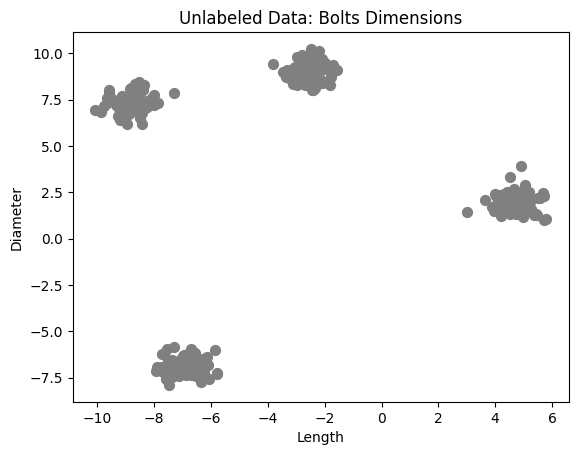
plt.scatter(X[:, 0], X[:, 1], c="gray", s=50)
plt.title("Unlabeled Data: Bolts Dimensions")
plt.xlabel("Length")
plt.ylabel("Diameter")
plt.show()

# Apply K-means Clustering
kmeans = KMeans(n_clusters=4, random_state=42)
y_kmeans = kmeans.fit_predict(X)

# Plot Clusters
plt.scatter(X[:, 0], X[:, 1], c=y_kmeans, cmap="viridis", s=50)
centers = kmeans.cluster_centers_
plt.scatter(centers[:, 0], centers[:, 1], c="red", s=200, alpha=0.75, marker="X")
plt.title("K-means Clustering of Bolts")
plt.xlabel("Length")
plt.ylabel("Diameter")
plt.show()

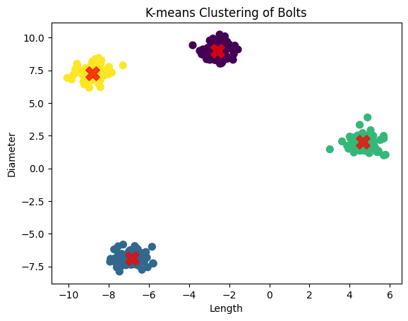
🔍 What You’ll Observe:

• The data is initially unlabeled.

• K-means clusters the bolts into 4 groups based on length and diameter.

• Cluster centers are marked with red ‘X’s.

🎈 Key Takeaway:

The model automatically groups similar bolts together, helping you identify different categories without any prior labels. Perfect for quality control in manufacturing! 🎉

📉 Dimensionality Reduction with PCA

High-dimensional data can be hard to visualize. Let’s use Principal Component Analysis (PCA) to reduce dimensions for visualization.

🔻 Example: Reducing Dimensions in Sensor Data

from sklearn.decomposition import PCA
from sklearn.datasets import load_iris

# Load example dataset
iris = load_iris()
X = iris.data
y = iris.target

# Apply PCA to reduce dimensions to 2
pca = PCA(n_components=2)
X_pca = pca.fit_transform(X)

# Plot the reduced data
plt.scatter(X_pca[:, 0], X_pca[:, 1], c=y, cmap="viridis", s=50)
plt.title("PCA - Dimensionality Reduction")
plt.xlabel("Principal Component 1")
plt.ylabel("Principal Component 2")
plt.show()

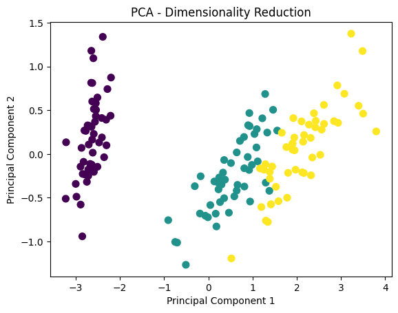
🔍 What You’ll Observe:

• Data is reduced to 2 dimensions, making it easier to visualize.

• You can still see clusters corresponding to different classes!

🎈 Key Takeaway:

PCA reduces the complexity of data while preserving patterns, making it useful for data visualization and noise reduction in engineering systems.

🚨 Anomaly Detection Example

Let’s detect anomalies in sensor data using Isolation Forest.

from sklearn.ensemble import IsolationForest

# Synthetic data: Normal and Anomalous readings
X = np.random.normal(0, 1, (100, 2))
X = np.concatenate([X, np.random.uniform(-4, 4, (10, 2))])  # Adding anomalies

# Apply Isolation Forest
iso_forest = IsolationForest(contamination=0.1, random_state=42)
y_pred = iso_forest.fit_predict(X)

# Plot the results
plt.scatter(X[:, 0], X[:, 1], c=y_pred, cmap="coolwarm", s=50)
plt.title("Anomaly Detection with Isolation Forest")
plt.xlabel("Sensor 1")
plt.ylabel("Sensor 2")
plt.show()

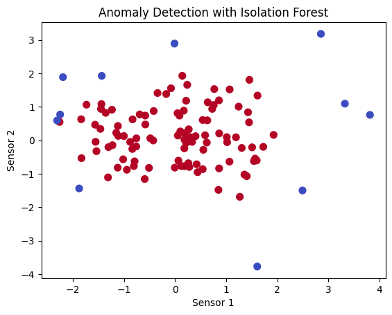
🔍 What You’ll Observe:

• Most data points are labeled as normal (blue).

• Anomalous points are identified as outliers (red).

🎈 Key Takeaway:

This method is excellent for fault detection and predictive maintenance, identifying unusual patterns that could indicate equipment failures.

🚀 Why Use Unsupervised Learning?

• No Labels Needed: Perfect for exploring uncharted data.

• Discover Hidden Patterns: Find clusters, anomalies, or trends you didn’t know existed.

• Data Preprocessing: Use Dimensionality Reduction to simplify complex datasets.

🎉 Key Takeaways

• Clustering: Grouping similar items together (e.g., K-means, Hierarchical Clustering).

• Dimensionality Reduction: Simplifying data while retaining essential patterns (e.g., PCA).

• Anomaly Detection: Identifying unusual data points (e.g., Isolation Forest).

• Goal: Discover insights and patterns without labeled data.

🌐 Where to Learn More?

• Scikit-learn Documentation

• Unsupervised Learning with Python

• Kaggle for hands-on datasets and competitions