📖 🌟 NumPy Guide 🌟

📖 🌟 NumPy Guide 🌟#

NumPy is a Python library that provides support for large, multi-dimensional arrays and matrices, along with a collection of mathematical functions to operate on these arrays. It is the fundamental package for scientific computing with Python. Even if you don’t explicitly use NumPy, it is likely that you are using it indirectly through other libraries like Pandas, Matplotlib, and SciPy. Nearly everything in the python data science ecosystem relies on NumPy.

🛠️ How to Import NumPy#

To start using NumPy, first, install it by following these instructions. After installation, import it into your Python script:

import numpy as np

Why np? This is the widely accepted alias for NumPy. Using np ensures that the library is easily accessible in your code and avoids conflicts with other modules.

🤔 Why Use NumPy?#

Why not just use Python lists?#

While Python lists are versatile and great for general-purpose programming, NumPy arrays offer significant performance benefits for numerical computations:

Memory Efficiency: NumPy arrays use less memory compared to lists.
Speed: Operations on NumPy arrays are faster than on lists because they are implemented in C.
Functionality: Provides a wide range of mathematical operations, such as linear algebra, Fourier transforms, and random number generation.

🔢 What is an “Array”?#

An array is a grid-like structure used to store data. It can have one or more dimensions:

1D Array (Vector): $$ \begin{array}{|c||c|c|c|} \hline 1 & 5 & 2 & 0 \\ \hline \end{array} $$
2D Array (Matrix): $$ \begin{array}{|c||c|c|c|} \hline 1 & 5 & 2 & 0 \\ \hline 8 & 3 & 6 & 1 \\ \hline 1 & 7 & 2 & 9 \\ \hline \end{array} $$
3D Array (Tensor): Think of this as a stack of 2D arrays.

🧩 Characteristics of NumPy Arrays:#

A NumPy array is a custom data structure, it is similar to a Python list but has some restrictions that allow it to be much more efficient for numerical computations, and have several built in methods that make it easier to work with.

Homogeneous Data: All elements must have the same data type.
Fixed Size: Once created, the array size cannot change.
Rectangular Shape: All rows must have the same number of columns in 2D arrays.

These restrictions make arrays more memory-efficient and faster for mathematical operations.

🏗️ Array Fundamentals#

🚀 Creating an Array#

You can create a NumPy array using Python lists:

a = np.array([1, 2, 3, 4, 5, 6])
a

array([1, 2, 3, 4, 5, 6])

Accessing elements:

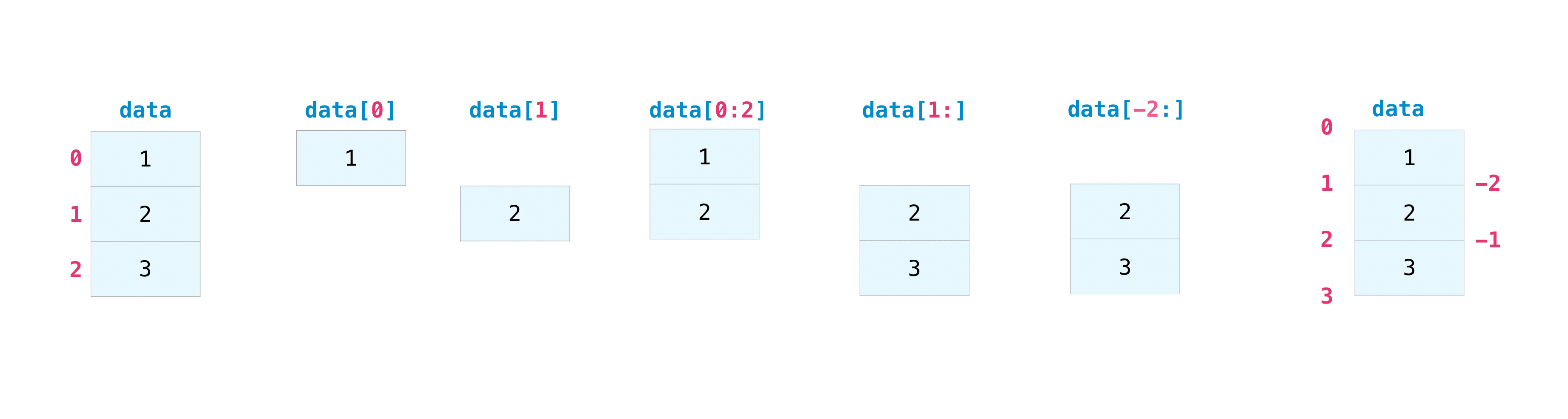
Elements in an array can be accessed using their index (starting from 0):

a[0]

np.int64(1)

Note

You can see that NumPy used dynamic typing to infer the data type of the array. In this case, it inferred that the array should be of type int64. What do you think would happen if we made one of the values 1.0? Try it out!

here is an example of some of the most common ways to index NumPy arrays:

Mutability: NumPy arrays are mutable, meaning you can modify their elements:

a[0] = 10
a

array([10,  2,  3,  4,  5,  6])

Here we change the value of the first element, the 0th index, in the array to 10.

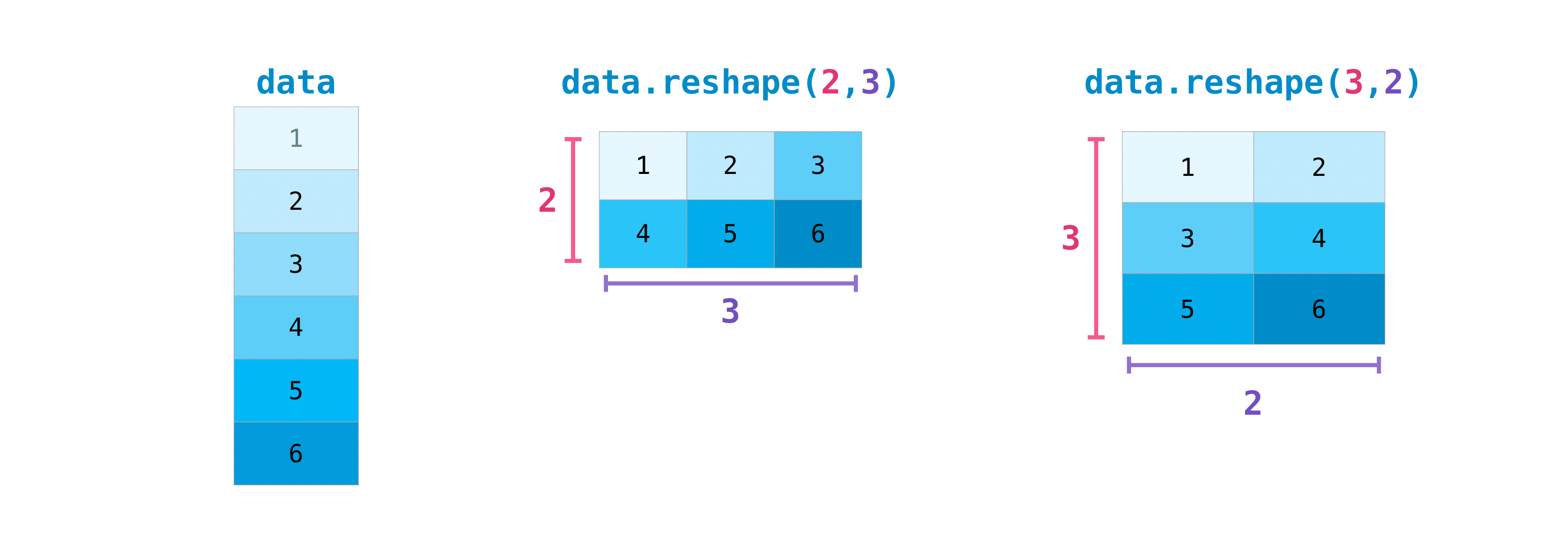
🔄 Reshaping Arrays#

Arrays can be reshaped without changing their data:

a = np.arange(6)
b = a.reshape(3, 2)
b

array([[0, 1],
       [2, 3],
       [4, 5]])

Note

The total number of elements must remain constant during reshaping. For example, a 2x3 array has 6 elements, so it can be reshaped into a 3x2 array or a 6x1 array, but not a 2x2 array.

🔍 Array Attributes#

Number of Dimensions: .ndim
Shape: .shape
Total Elements: .size
Data Type: .dtype

Example:

a = np.array([[1, 2, 3], [4, 5, 6]])
a.ndim  # Number of dimensions

a.shape  # Shape of the array

(2, 3)

a.size  # Total number of elements

a.dtype  # Data type of elements

dtype('int64')

🧮 Mathematical Operations#

NumPy allows you to perform operations like addition, subtraction, and multiplication on arrays directly:

a = np.array([1, 2, 3, 4])
b = np.array([5, 6, 7, 8])

# Element-wise addition
a + b

array([ 6,  8, 10, 12])

# Element-wise multiplication
a * b

array([ 5, 12, 21, 32])

# Sum of all elements
a.sum()

np.int64(10)

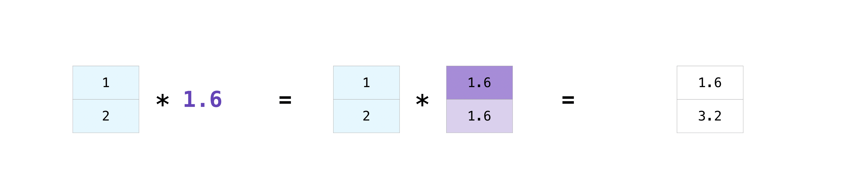
📊 Broadcasting#

Broadcasting allows you to perform operations between arrays of different shapes:

a = np.array([1, 2, 3])
a + 5  # Add 5 to every element

array([6, 7, 8])

When you apply an operation between an array and a scalar, numpy uses broadcasting to apply the operation to each element of the array.

Note

The shapes of the arrays must be compatible for broadcasting.

🏆 Finding Maximum and Minimum Values#

NumPy provides efficient built-in methods for finding the maximum and minimum values in an array.

np.max(): Returns the maximum value of an array or along a specific axis.
np.min(): Returns the minimum value of an array or along a specific axis.
np.argmax() and np.argmin(): Return the indices of the maximum and minimum values.

data = np.array([[3, 7, 1], [4, 5, 9]])

# Find global max and min
np.max(data)

np.int64(9)

np.min(data)

np.int64(1)

# Find max and min along rows (axis=1)
np.max(data, axis=1)

array([7, 9])

np.min(data, axis=1)

array([1, 4])

# Find the indices of max and min
np.argmax(data)  # Global index of max value

np.int64(5)

np.argmin(data)  # Global index of min value

np.int64(2)

Tip

Combine these methods for advanced analysis. For example, use np.unravel_index() with argmax/argmin to find the row and column of the max/min in a multi-dimensional array.

🧰 Preallocation of Memory#

Preallocating memory for large arrays is a good practice when working with performance-critical applications. Instead of dynamically appending to lists (which is slow), create an empty array or an array filled with default values like zeros or ones.

Preallocation Methods:#

np.zeros(shape): Creates an array filled with zeros.
np.ones(shape): Creates an array filled with ones.
np.empty(shape): Creates an uninitialized array (faster, but contains arbitrary values).
np.full(shape, fill_value): Creates an array filled with a specific value.

# Preallocate an array of zeros
zeros = np.zeros((3, 3))
zeros

array([[0., 0., 0.],
       [0., 0., 0.],
       [0., 0., 0.]])

# Preallocate an array of ones
ones = np.ones((2, 4))
ones

array([[1., 1., 1., 1.],
       [1., 1., 1., 1.]])

# Preallocate an uninitialized array
uninit = np.empty((2, 2))
uninit

array([[4.9e-324, 9.9e-324],
       [1.5e-323, 2.0e-323]])

# Preallocate an array filled with 42
filled = np.full((3, 3), 42)
filled

array([[42, 42, 42],
       [42, 42, 42],
       [42, 42, 42]])

Tip

When to Use Preallocation:

np.zeros() and np.ones() are great for initializing arrays for numerical computations.
np.empty() is ideal when you’ll overwrite all values in the array soon after creation.
Preallocation prevents the overhead of dynamically resizing arrays during iterative operations.

🔢 Sorting Arrays#

NumPy makes sorting arrays simple and efficient with the np.sort() method and related functions.

Key Sorting Functions:#

np.sort(): Returns a sorted copy of the array.
np.argsort(): Returns the indices that would sort the array.
np.lexsort(): Sorts based on multiple keys.
np.partition(): Partially sorts the array by selecting elements up to a specific index.

data = np.array([3, 1, 4, 1, 5, 9])

# Sort the array in ascending order
np.sort(data)

array([1, 1, 3, 4, 5, 9])

# Get the indices that would sort the array
np.argsort(data)

array([1, 3, 0, 2, 4, 5])

# Sort a 2D array along rows (default axis=1)
matrix = np.array([[5, 2, 9], [3, 7, 1]])
np.sort(matrix)

array([[2, 5, 9],
       [1, 3, 7]])

# Sort along columns (axis=0)
np.sort(matrix, axis=0)

array([[3, 2, 1],
       [5, 7, 9]])

Tip

Advanced Sorting: Use np.lexsort() to sort by multiple keys.

names = np.array(["Alice", "Bob", "Charlie"])
scores = np.array([85, 95, 85])

# Sort by scores, then names
idx = np.lexsort((names, scores))
idx

array([0, 2, 1])

names[idx]

array(['Alice', 'Charlie', 'Bob'], dtype='<U7')

🔗 Finding Unique Elements#

NumPy provides np.unique() for identifying unique elements in an array. You can also retrieve additional information, such as indices or counts.

Key Features of `np.unique()`:#

Find unique elements: Returns the sorted unique elements in the array.
Return indices: Identify the positions of unique elements in the original array.
Return counts: Count occurrences of unique elements.

data = np.array([1, 2, 2, 3, 3, 3, 4, 4, 4, 4])

# Find unique elements
np.unique(data)

array([1, 2, 3, 4])

# Return unique elements with their counts
unique_elements, counts = np.unique(data, return_counts=True)
unique_elements

array([1, 2, 3, 4])

counts

array([1, 2, 3, 4])

# Return indices of the first occurrences
unique_elements, indices = np.unique(data, return_index=True)
indices

array([0, 1, 3, 6])

Unique in 2D Arrays#

By default, np.unique() flattens the input array. Use the axis parameter to find unique rows or columns.

matrix = np.array([[1, 2], [3, 4], [1, 2]])

# Unique rows
np.unique(matrix, axis=0)

array([[1, 2],
       [3, 4]])

Tip

Use return_counts=True to analyze frequency distributions in datasets, useful for exploratory data analysis.

Summary of Methods#

Function	Purpose
`np.max()` / `np.min()`	Maximum/minimum value of an array
`np.argmax()` / `np.argmin()`	Indices of maximum/minimum values
`np.zeros()` / `np.ones()`	Preallocate arrays with zeros or ones
`np.empty()`	Preallocate an uninitialized array
`np.sort()`	Return a sorted array
`np.argsort()`	Return indices to sort the array
`np.lexsort()`	Sort based on multiple keys
`np.unique()`	Find unique elements, indices, and counts

🎲 Random Number Generation#

Generate random numbers for simulations or initializing models:

rng = np.random.default_rng()
rng.random(5)  # 5 random numbers between 0 and 1

array([0.55209632, 0.78196038, 0.66513899, 0.48235682, 0.74998171])

For random integers:

rng.integers(10, size=(2, 3))  # Random integers from 0 to 9

array([[7, 7, 9],
       [2, 4, 1]])

📂 Saving and Loading Data#

Binary Format:#

Binary files are faster to read and write compared to text files.

Save:

np.save("array.npy", a)

Load:

b = np.load("array.npy")
b

array([1, 2, 3])

Text Format:#

Text files are human-readable and can be opened in any text editor.

Save as CSV:

np.savetxt("array.csv", a, delimiter=",")

Load from CSV:

c = np.loadtxt("array.csv", delimiter=",")
c

array([1., 2., 3.])

📖 Getting Help#

Need help with NumPy functions? Use Python’s built-in help() function or IPython’s ?:

help(np.array)  # Built-in documentation

Help on built-in function array in module numpy:

array(...)
    array(object, dtype=None, *, copy=True, order='K', subok=False, ndmin=0,
          like=None)
    
    Create an array.
    
    Parameters
    ----------
    object : array_like
        An array, any object exposing the array interface, an object whose
        ``__array__`` method returns an array, or any (nested) sequence.
        If object is a scalar, a 0-dimensional array containing object is
        returned.
    dtype : data-type, optional
        The desired data-type for the array. If not given, NumPy will try to use
        a default ``dtype`` that can represent the values (by applying promotion
        rules when necessary.)
    copy : bool, optional
        If ``True`` (default), then the array data is copied. If ``None``,
        a copy will only be made if ``__array__`` returns a copy, if obj is
        a nested sequence, or if a copy is needed to satisfy any of the other
        requirements (``dtype``, ``order``, etc.). Note that any copy of
        the data is shallow, i.e., for arrays with object dtype, the new
        array will point to the same objects. See Examples for `ndarray.copy`.
        For ``False`` it raises a ``ValueError`` if a copy cannot be avoided.
        Default: ``True``.
    order : {'K', 'A', 'C', 'F'}, optional
        Specify the memory layout of the array. If object is not an array, the
        newly created array will be in C order (row major) unless 'F' is
        specified, in which case it will be in Fortran order (column major).
        If object is an array the following holds.
    
        ===== ========= ===================================================
        order  no copy                     copy=True
        ===== ========= ===================================================
        'K'   unchanged F & C order preserved, otherwise most similar order
        'A'   unchanged F order if input is F and not C, otherwise C order
        'C'   C order   C order
        'F'   F order   F order
        ===== ========= ===================================================
    
        When ``copy=None`` and a copy is made for other reasons, the result is
        the same as if ``copy=True``, with some exceptions for 'A', see the
        Notes section. The default order is 'K'.
    subok : bool, optional
        If True, then sub-classes will be passed-through, otherwise
        the returned array will be forced to be a base-class array (default).
    ndmin : int, optional
        Specifies the minimum number of dimensions that the resulting
        array should have.  Ones will be prepended to the shape as
        needed to meet this requirement.
    like : array_like, optional
        Reference object to allow the creation of arrays which are not
        NumPy arrays. If an array-like passed in as ``like`` supports
        the ``__array_function__`` protocol, the result will be defined
        by it. In this case, it ensures the creation of an array object
        compatible with that passed in via this argument.
    
        .. versionadded:: 1.20.0
    
    Returns
    -------
    out : ndarray
        An array object satisfying the specified requirements.
    
    See Also
    --------
    empty_like : Return an empty array with shape and type of input.
    ones_like : Return an array of ones with shape and type of input.
    zeros_like : Return an array of zeros with shape and type of input.
    full_like : Return a new array with shape of input filled with value.
    empty : Return a new uninitialized array.
    ones : Return a new array setting values to one.
    zeros : Return a new array setting values to zero.
    full : Return a new array of given shape filled with value.
    copy: Return an array copy of the given object.
    
    
    Notes
    -----
    When order is 'A' and ``object`` is an array in neither 'C' nor 'F' order,
    and a copy is forced by a change in dtype, then the order of the result is
    not necessarily 'C' as expected. This is likely a bug.
    
    Examples
    --------
    >>> import numpy as np
    >>> np.array([1, 2, 3])
    array([1, 2, 3])
    
    Upcasting:
    
    >>> np.array([1, 2, 3.0])
    array([ 1.,  2.,  3.])
    
    More than one dimension:
    
    >>> np.array([[1, 2], [3, 4]])
    array([[1, 2],
           [3, 4]])
    
    Minimum dimensions 2:
    
    >>> np.array([1, 2, 3], ndmin=2)
    array([[1, 2, 3]])
    
    Type provided:
    
    >>> np.array([1, 2, 3], dtype=complex)
    array([ 1.+0.j,  2.+0.j,  3.+0.j])
    
    Data-type consisting of more than one element:
    
    >>> x = np.array([(1,2),(3,4)],dtype=[('a','<i4'),('b','<i4')])
    >>> x['a']
    array([1, 3], dtype=int32)
    
    Creating an array from sub-classes:
    
    >>> np.array(np.asmatrix('1 2; 3 4'))
    array([[1, 2],
           [3, 4]])
    
    >>> np.array(np.asmatrix('1 2; 3 4'), subok=True)
    matrix([[1, 2],
            [3, 4]])

np.array?

For even more details, use ??:

np.array??

🧑‍🏫 Working with Mathematical Formulas#

NumPy simplifies mathematical operations on arrays. For example, the Mean Squared Error (MSE) formula:

\[ \text{MSE} = \frac{1}{n} \sum_{i=1}^{n} (y_i - \hat{y}_i)^2 \]

Implementation in NumPy:

labels = np.array([1, 2, 3])
predictions = np.array([1.1, 1.9, 3.2])
mse = np.mean((labels - predictions) ** 2)
mse

np.float64(0.020000000000000035)

🧮 Advanced Mathematical Operations in NumPy#

NumPy is packed with mathematical tools for handling arrays, from basic arithmetic to more advanced mathematical operations. Here’s an overview of the most useful ones:

1️⃣ Basic Element-Wise Operations#

NumPy performs operations element-wise by default. You can add, subtract, multiply, or divide arrays easily:

a = np.array([1, 2, 3, 4])
b = np.array([5, 6, 7, 8])

# Addition
a + b

array([ 6,  8, 10, 12])

# Subtraction
a - b

array([-4, -4, -4, -4])

# Multiplication
a * b

array([ 5, 12, 21, 32])

# Division
a / b

array([0.2       , 0.33333333, 0.42857143, 0.5       ])

Note

If you combine arrays of different shapes, NumPy will attempt broadcasting.

2️⃣ Power and Exponentials#

Exponentiation: Use np.exp() to compute the exponential of all elements in the array.
Powers: Raise elements to a power using np.power() or the ** operator.
Logarithms: Use np.log() for natural log, np.log10() for base-10 log.

x = np.array([1, 2, 3, 4])

# Exponential
np.exp(x)

array([ 2.71828183,  7.3890561 , 20.08553692, 54.59815003])

# Powers
np.power(x, 3)  # Cube every element

array([ 1,  8, 27, 64])

# Natural log
np.log(x)

array([0.        , 0.69314718, 1.09861229, 1.38629436])

# Base-10 log
np.log10(x)

array([0.        , 0.30103   , 0.47712125, 0.60205999])

3️⃣ Trigonometric Functions#

NumPy supports trigonometric functions like sine, cosine, and tangent. All angles are in radians by default.

angles = np.array([0, np.pi / 2, np.pi])

# Sine
np.sin(angles)

array([0.0000000e+00, 1.0000000e+00, 1.2246468e-16])

# Cosine
np.cos(angles)

array([ 1.000000e+00,  6.123234e-17, -1.000000e+00])

# Tangent
np.tan(angles)

array([ 0.00000000e+00,  1.63312394e+16, -1.22464680e-16])

Other trigonometric methods include:

np.arcsin(), np.arccos(), np.arctan() for inverse trigonometric functions.
np.deg2rad() and np.rad2deg() for converting between degrees and radians.

4️⃣ Statistics#

NumPy provides many statistical methods for arrays:

np.mean(): Mean (average).
np.median(): Median.
np.std(): Standard deviation.
np.var(): Variance.
np.min() and np.max(): Minimum and maximum values.
np.percentile(): Compute the nth percentile.

data = np.array([1, 2, 3, 4, 5])

# Mean
np.mean(data)

np.float64(3.0)

# Median
np.median(data)

np.float64(3.0)

# Standard deviation
np.std(data)

np.float64(1.4142135623730951)

# Variance
np.var(data)

np.float64(2.0)

# Percentile
np.percentile(data, 50)  # Median

np.float64(3.0)

5️⃣ Linear Algebra#

Linear algebra operations are critical for many engineering and scientific applications. NumPy provides np.linalg for this purpose:

Tip

If you are currently enrolled in a linear algebra course, you can use NumPy to check your answers.

# Define a 2D matrix
matrix = np.array([[1, 2], [3, 4]])

# Transpose
matrix.T

array([[1, 3],
       [2, 4]])

# Matrix Multiplication
np.dot(matrix, matrix)

array([[ 7, 10],
       [15, 22]])

# Determinant
np.linalg.det(matrix)

np.float64(-2.0000000000000004)

# Eigenvalues and Eigenvectors
eigvals, eigvecs = np.linalg.eig(matrix)

print("eignvalues: ", eigvals)
print("eigenvectors: ", eigvecs)

eignvalues:  [-0.37228132  5.37228132]
eigenvectors:  [[-0.82456484 -0.41597356]
 [ 0.56576746 -0.90937671]]

Additional methods:

np.linalg.inv(): Matrix inverse.
np.linalg.norm(): Vector or matrix norm.
np.linalg.qr(): QR decomposition.
np.linalg.svd(): Singular Value Decomposition (SVD).

6️⃣ Sorting and Searching#

Sorting: Use np.sort() to sort elements in ascending order.
Search for Elements: Use np.where() to find indices of elements that match a condition.

data = np.array([3, 1, 4, 1, 5])

# Sort the array
np.sort(data)

array([1, 1, 3, 4, 5])

# Find indices of elements greater than 3
np.where(data > 3)

(array([2, 4]),)

7️⃣ Aggregations#

Aggregate methods operate along entire arrays or specified axes:

np.sum(): Sum of elements.
np.prod(): Product of elements.
np.cumsum(): Cumulative sum.
np.cumprod(): Cumulative product.

data = np.array([1, 2, 3, 4])

# Sum of all elements
np.sum(data)

np.int64(10)

# Product of all elements
np.prod(data)

np.int64(24)

# Cumulative sum
np.cumsum(data)

array([ 1,  3,  6, 10])

# Cumulative product
np.cumprod(data)

array([ 1,  2,  6, 24])

8️⃣ Clipping and Rounding#

Clipping: Restrict array values within a range using np.clip().
Rounding: Round values using np.round(), np.floor(), np.ceil(), etc.

data = np.array([1.2, 2.5, 3.7, 4.4])

# Clip values between 2 and 4
np.clip(data, 2, 4)

array([2. , 2.5, 3.7, 4. ])

# Round values
np.round(data)

array([1., 2., 4., 4.])

# Floor and Ceil
np.floor(data)  # Round down

array([1., 2., 3., 4.])

np.ceil(data)  # Round up

array([2., 3., 4., 5.])

9️⃣ Random Sampling#

Use np.random to generate random values for simulations:

np.random.random(): Uniform random values.
np.random.normal(): Random values from a normal distribution.
np.random.randint(): Random integers within a range.

# Random values between 0 and 1
np.random.random(5)

array([0.39325984, 0.67202451, 0.75823814, 0.53178579, 0.43872361])

# Random integers between 10 and 20
np.random.randint(10, 20, size=5)

array([15, 18, 15, 13, 16])

These mathematical tools make NumPy the backbone of scientific computing in Python. With these methods, you can efficiently handle numerical data for any engineering, research, or data science task! 🚀

📖 🌟 NumPy Guide 🌟

Contents

📖 🌟 NumPy Guide 🌟#

🛠️ How to Import NumPy#

🤔 Why Use NumPy?#

Why not just use Python lists?#

🔢 What is an “Array”?#

🧩 Characteristics of NumPy Arrays:#

🏗️ Array Fundamentals#

🚀 Creating an Array#

🔄 Reshaping Arrays#

🔍 Array Attributes#

🧮 Mathematical Operations#

📊 Broadcasting#

🏆 Finding Maximum and Minimum Values#

🧰 Preallocation of Memory#

Preallocation Methods:#

🔢 Sorting Arrays#

Key Sorting Functions:#

🔗 Finding Unique Elements#

Key Features of np.unique():#

Unique in 2D Arrays#

Summary of Methods#

🎲 Random Number Generation#

📂 Saving and Loading Data#

Binary Format:#

Text Format:#

📖 Getting Help#

🧑‍🏫 Working with Mathematical Formulas#

🧮 Advanced Mathematical Operations in NumPy#

1️⃣ Basic Element-Wise Operations#

2️⃣ Power and Exponentials#

3️⃣ Trigonometric Functions#

4️⃣ Statistics#

5️⃣ Linear Algebra#

6️⃣ Sorting and Searching#

7️⃣ Aggregations#

8️⃣ Clipping and Rounding#

9️⃣ Random Sampling#

Key Features of `np.unique()`:#